Below is an annotated version of the script objective_analysis_demo.jnl
! objective_analysis_demo.jnl (4/99)

! Description: Demonstration of interpolating scattered data
to grids

! External Functions introduced in Ferret V5.0
! Two interpolation techniques are available for gridding.

! Note that both of these are applicable ONLY for output
! grids which are REGULAR, that is to say, have EQUALLY-SPACED
! coordinates.

! Here we set up viewports and an abstract mathematical function
to demonstrate the gridding technique.
|
! Set viewports DEFINE VIEW/ylim=.6,1/text=.5 vupper DEFINE VIEW/xlim=0.,.5/ylim=.3,.55/text=.2 vul DEFINE VIEW/xlim=.5,1./ylim=.3,.55/text=.2 vur DEFINE VIEW/xlim=0.,.5/ylim=0.05,.3/text=.2 vll DEFINE VIEW/xlim=.5,1./ylim=0.05,.3/text=.2 vlr ! Define a 2-dimensional function and sample it DEFINE AXIS/x=0:10:0.05 x10 DEFINE AXIS/y=0:10:0.05 y10 DEFINE GRID/x=x10/y=y10 g10x10 SET GRID g10x10 LET WAVE = SIN(KX*XPTS + KY*YPTS - PHASE) / 3 LET PHASE = 0 LET KAPPA = 0.4 LET KX = 0.4 LET KY = 0.7 LET FCN1 = SIN(R)/(R+1) LET R = ((XPTS-X0)^2+ 5*(YPTS-Y0)^2)^0.5 LET X0 = 3 LET Y0 = 8 LET sample_function = fcn1 + wave |
For simplicity this demo will work with abstract mathematical functions rather than with "real" data. We will create an abstract function in the XY plane and use it as a model of "reality". Our goal is to sample this "reality" at scattered (X,Y) points and then attempt to recreate the original field through interpolation and objectibe analysis techniques.
From here on the lines you see will be exactly the lines executed in this demonstration script. To focus attention on the issues of regridding and avoid the clutter of graphics layout commands you will notice that graphics are performed by a script called "draw_it".
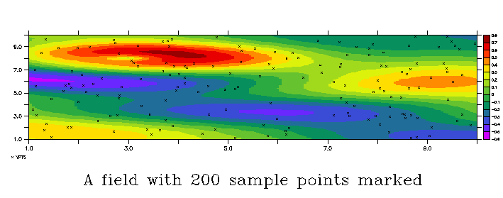
! **********************************************************
! To display "reality" we will first let our sample points (xpts,ypts) be
! simply the X and y points of a grid.  Then we will change (xpts,ypts) to
! be 200 sampling locations and mark them with symbols on the plot.
! We will draw this output in the "upper" viewport.  The script draw_it
! simplifies plotting the functions in a viewport and with a title.

! Shaded plot of the points on the (X,Y) grid
|
LET xpts = x; LET ypts = y GO draw_it "fcn1+wave" "A field with 200 sample points marked" "SHADE" upper ! points randomly sampled in (X,Y) LET xpts = 10*randu(i); LET ypts = 10*randu(i+2) SET REGION/i=1:200 PLOT/VS/OVER/SYMBOLS xpts,ypts |
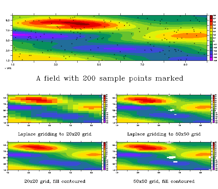
! **********************************************************
! Now we will interpolate those 200 (X,Y,value) triples back onto a regular
! grid in the (X,Y) plane.  The output grid will be from 1 to 10 by .5 along
! both the X and y axes.  Defaults will be used for the interpolation controls.
!
! Under the "SHADEd" (raster-style) plot we will display the very same result
! as a filled contour.
|
! Define regularly-spaced output axes DEFINE AXIS/x=1:10:.5 xax5 DEFINE AXIS/y=1:10:.5 yax5 LET sgrid = scat2gridlaplace_xy (xpts, ypts, sample_function, x[gx=xax5], y[gy=yax5], 5., 5) GO draw_it sgrid "Interpolated w/ ext fcn to 20x20 grid" "SHADE" upper_left GO draw_it sgrid "20x20 grid, fill contoured" "FILL" lower_left |

! **********************************************************
! Now we perform the identical analysis but we will interpolate onto a
! higher resolution grid.  The gaps in the output are because there are
! points on this output grid that are unacceptably far from any sample
! points using these interpolation parameters.
|
! Define regularly-spaced output axes DEFINE AXIS/x=1:10:.2 xax2 DEFINE AXIS/y=1:10:.2 yax2 LET sgrid = scat2gridlaplace_xy (xpts, ypts, sample_function, x[gx=xax2], y[gy=yax2], 5., 5) GO draw_it sgrid "Interpolated w/ ext fcn to 50x50 grid" "SHADE" upper_right GO draw_it sgrid "50x50 grid, fill contoured" "fill" lower_right |
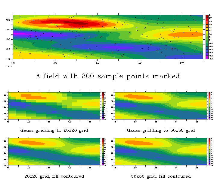
! Now do the same plots with the Gaussian gridding function
! scat2gridgauss_xy which uses a different technique to interpolate the
! scattered points to the grid.  This results in a somewhat smoother plot.
! The interpolation parameters are  XSCALE, YSCALE, XCUTOFF, YCUTOFF;
! where the algorithm uses scattered points which are within
!         cutoff* the scale width from the gridbox center.  We use
! XSCALE = YSCALE = 1; XCUTOFF = YCUTOFF = 2.
|
! Define regularly-spaced output axes DEFINE AXIS/x=1:10:.5 xax5 DEFINE AXIS/y=1:10:.5 yax5 LET/QUIET sgrid = scat2gridgauss_xy (xpts, ypts, sample_function, x[gx=xax5], y[gy=yax5], 1.,1.,2.,2) GO draw_it sgrid "Gauss gridding to 20x20 grid" "SHADE" upper_left GO draw_it sgrid "20x20 grid, fill contoured" "FILL" lower_left DEFINE AXIS/x=1:10:.2 xax2 DEFINE AXIS/y=1:10:.2 yax2 LET/QUIET sgrid = scat2gridgauss_xy (xpts, ypts, sample_function, x[gx=xax2], y[gy=yax2], 1.,1.,2.,2) GO draw_it sgrid "Gauss gridding to 50x50 grid" "SHADE" upper_right GO draw_it sgrid "50x50 grid, fill contoured" "fill" lower_right |
This demo replaces pre_V50_objective_analysis_demo.jnl
NOTE
A set of new functions (February 2005) return the number of scattered points contained in each output grid cell. The functions are named scatgrid_nobs_xy, scatgrid_nobs_xz, and so forth. They are called as follows:
yes? LET a = SCATGRID_NOBS_XY(xpts, ypts, xout, yout)where xpts and ypts are the coordinates of the scattered points to be gridded, and xout and yout are variables which have the X and Y axes of the output grid. The result is on the xout, yout grid and at each x,y contains a count of the scattered points in that output grid cell. This count is independent of the gridding function that may be called in a separate step (Gaussian or Laplace method); it relates the scattered point to the grid we will interpolate them onto. These functions will be part of a future release of Ferret (after version 5.80 released in January 2005). To obtain them now, please download this tar file, which contains the source code and pre-compiled shared object files for linux RH9, Solaris 5.6 and Solaris 5.8.
If you need a set of compiled functions for another operating system please either set yourself up to compile external functions as explained on the External Functions webpage (it isn't difficult!), or contact the Ferret developers at oar.pmel.contact_ferret@noaa.gov and we'll see what we can do.