Ferret Version 5.8 Release Notes

January 3, 2005

New Features and Enhancements in Version 5.8

Functions to regrid data from a curvilinear grid to a rectilinear grid
Function to regrid data from a rectilinear grid to a curvilinear grid
Optimization of some operations
Allow for different scale and offset values inside each stepfile of a multi-file data set
New color palette files, including ones designed for color-impaired viewers
New symbols are defined for all plots, detailing the current viewport settings

New Documentation

New FAQ: How can I show the value of my variable at its deepest depth?
New FAQ: Can I use Ferret to draw a Taylor Diagram?
New FAQ: How can I plot a subset of my curvilinear data?
New FAQ: Which of Ferret's color palettes best convey information to color-impaired viewers?

Minor Syntax Changes in Version 5.8

Change in the message returned on an error in a GO script argument
PLOT/THICK without a color specifier now cycles through colors for lines
PPL POLYGON is allowed as well as PPL FILLPOL

Bug Fixes in Version 5.8

Within a script, $0 returns the script name.
Bug with long labels and multi-line labels with the <NL> line separator
The result of the COMPRESSK function did not vary in X
Fixed a bug in POLYGON (or SHADE) plots with a single level
Changes to colorbar labels
Fixed format of coordinates listed with LIST/FORMAT=tab or /FORMAT=comma
Changing pen with @Cnnn in multi-line labels
(Under linux only), var[d=filename] failed if filename starts with a digit
Label the complete OPeNDAP (DODS) URL
Error when /HLMITS qualifier resulted in in a span containing just one coordinate point
Illegal value of 0 in a stride crashed Ferret
Regridding with @NRST between two different calendar axes
Bug overlaying a polygon on a non-Gregorian time axis is fixed
list commands and missing-data of NaN

New Features and Enhancements in Version 5.8

Functions to regrid data from a curvilinear grid to a rectilinear grid
The function CURV_TO_RECT_MAP uses spherical interpolation to compute the mapping from a curvilinear grid to a rectilinear grid defined in Ferret. Once this mapping is computed, use the function CURV_TO_RECT to apply the map to any number of variables, regridding them to the output grid. This sequence lets us compare data from models and observations, or models with one another. The output grid may be regularly spaced or irregularly spaced.

The functions are:

CURV_TO_RECT_MAP(lon_in,lat_in,grid_out,radius)
    Compute mapping for spherical interpolation: curvilinear to rectangular grid.
    lon_in: Source grid longitudes (2-D) (degrees)
    lat_in: Source grid latitudes (2-D) (degrees)
    grid_out: Any variable on destination Longitude-Latitude grid, Lon and Lat (degrees)
    radius: Source points falling within radius are included in mapping to destination point (degrees)

CURV_TO_RECT(V,mapping)
    Apply spherical interpolation: curvilinear to rectangular grid
    V: Variable to regrid, on curvilinear grid V(x,y,z,t)
    mapping: mapping computed by CURV_TO_RECT_MAP

For example:

   yes? USE "data/model_out.nc"  ! data with curvilinear coordinates
   
   yes? SHOW data
   currently SET data sets:
       1> /home/ansley/data/model_out.nc  (default)
    name     title             I         J         K         L
    LON   longitude of cell   1:180     1:173     ...       ...
    LAT   latitude of cell    1:180     1:173     ...       ...
    U     zonal wind          1:180     1:173     ...       ...
    V     meridional wind     1:180     1:173     ...       ...
   
   
   yes? LET lonin = lon[D=1]
   yes? LET latin = lat[D=1]
   
   yes? ! Define output grid and a variable on the output grid
   
   yes? DEF AXIS/X=0:355:5/MODULO/UNITS=degrees xax
   yes? DEF AXIS/Y=-90:90:5/UNITS=degrees yax
   yes? LET lonlatout = x[gx=xax] + y[gy=yax] 
   
   yes? ! Compute mapping, save to a file (computing mapping is slow)
   
   yes? LET radius = 10.
   yes? LET map = curv_to_rect_map ( lonin, latin, lonlatout, radius)
   yes? SAVE/CLOBBER/FILE=map_5deg.nc map  
   
   yes? ! Apply mapping to variables
   yes? CANCEL VAR/ALL
   yes? USE map_5deg.nc
   yes? LET regridded_u = curv_to_rect(U[D=1], map[D=2])
   yes? LET regridded_v = curv_to_rect(V[D=1], map[D=2])

These functions are implemented as an external function, and is only available on systems where external functions (shared object files) are available. It will be made an internally-linked function in future versions.

Function to regrid data on a rectilinear grid to a curvilinear grid.
The function RECT_TO_CURV uses bilinear interpolation to regrid data from a rectilinear grid to a curvilinear grid. Put any data on rectangular data onto model grids for comparison. This function takes much less computation than CURV_TO_RECT_MAP.

The function is:

RECT_TO_CURV(V,lon_bounds_out,lat_bounds_out,missing values allowed)
    bilinear interpolation from rectangular grid to curvilinear grid
    V: variable V(x,y,z,t) on rectilinear grid
    lon_bounds_out: Destination curvilinear grid longitude bounds(2-D) (degrees)
    lat_bounds_out: Destination curvilinear grid latitude bounds(2-D) (degrees)
    missing values allowed: number of missing values allowed in 4 surrounding source cells: 0 to 3

For example, compare model data to COADS_CLIMATOLOGY data:

   yes? USE "data/model_out.nc"
   yes? USE coads_climatology
   
   yes? SHOW data
   currently SET data sets:
       1> /home/ansley/data/model_out.nc  
    name     title             I         J         K         L
    LON   longitude of cell   1:180     1:173     ...       ...
    LAT   latitude of cell    1:180     1:173     ...       ...
    U     zonal wind          1:180     1:173     ...       ...
    V     merional wind       1:180     1:173     ...       ...
   
       2> /home/ja9/tmap/fer_dsets/data/coads_climatology.cdf  (default)
    name     title                             I         J         K         L
    SST      SEA SURFACE TEMPERATURE          1:180     1:90      ...       1:12
    AIRT     AIR TEMPERATURE                  1:180     1:90      ...       1:12
    SPEH     SPECIFIC HUMIDITY                1:180     1:90      ...       1:12
    WSPD     WIND SPEED                       1:180     1:90      ...       1:12
    UWND     ZONAL WIND                       1:180     1:90      ...       1:12
    VWND     MERIDIONAL WIND                  1:180     1:90      ...       1:12
    SLP      SEA LEVEL PRESSURE               1:180     1:90      ...       1:12

 
    yes? LET uwnd_curv = RECT_TO_CURV(uwnd[D=2,L=1], lon[D=1], lat[D=1], 1)
    yes? LET uwnd_diff = u[D=1] - uwnd_curv[D=2,L=1]

    ! Do a curvilinear shade plot of the difference.

    yes? SHADE uwnd_diff, lon[D=1], lat[D=1]

This function is implemented as an external function, and is only available on systems where external functions (shared object files) are available. It will be made an internally-linked function in future versions.

Some operations are optimized for better performance. Internal string operations, such as looking for a variable to see whether it is defined, or looking for a dataset or axis name, are done more efficiently. Scripts that use large large numbers of operations such as DEFINE VARIABLE (LET), or grave-accent expressions (immediate-mode evaluation) may significantly speed up. Here is a simple example, which in our tests runs up to four times faster in version 5.8 compared with version 5.7 of Ferret:
```
   yes? can mode verify
   yes? repeat/k=1:500 (let/quiet test`k` = `k`)
```

Allow different offset and scale attributes inside each stepfile within a multi-file dataset. Ferret reads the scale and offset before reading the data from each file, and applies the new scale and offset values as it reads the data. Note that the commands
```
yes? SAY `var, RETURN=nc_offset` 
yes? SAY `var, RETURN=nc_scale`
```
return the latest scale and offset value that were applied.

New color palette files, including ones designed for color-impaired viewers. A discussion of these new palettes with examples is in the FAQ, Which of Ferret's color palettes best convey information to color-impaired viewers? http://ferret.pmel.noaa.gov/static/FAQ/graphics/color_friendly_palettes.html
New symbols are defined for all plots, giving access to details of the current viewport settings. These are set for user-defined viewports and also for pre-defined viewports as in the command
```
   yes? set viewport right
```
Thew new symbols are: VP_SCALE, VP_XLO, VP_XHI, VP_YLO, VP_YHI, VP_RT_MARGIN, and VP_TOP_MARGIN. and they are defined as follows.

When a viewport is defined by a command like:
```
   yes? DEFINE VIEWPORT/XLIM=xlo:xyi/YLIM=ylo:yhi/TEXT=n  my_viewport 
   yes? SET VIEW my_viewport
```
The symbols VP_XLO, VP_XHI, VP_YLO, and VP_YHI are the arguments to /XLIM and /YLIM.
VP_SCALE is related to the DEFINE VIEWPORT/TEXT qualifier, if used, or to the default scaling if /TEXT is not used in the viewport definition. See the explanation in the section on DEFINE VIEWPORT in the Users Guide.
VP_RT_MARGIN and VP_TOP_MARGIN are the space remaining on the page at the right and the top, beyond the ends of the x and y axes; PPL$XORG and PPL$YORG are symbols that already give us the left and bottom margin sizes.

Minor Syntax Changes in Version 5.8

Change in the message returned on an error in a GO script argument. We have changed the message "*** NOTE" to "** ERROR". In GO scripts, arguments are checked with the QUERY/IGNORE command. If the argument test fails, Ferret previously returned text preceded by "** NOTE". Ferret then returns to the command line. It is more consistent with other Ferret error handling to return the "** ERROR" text, since the behavior of QUERY is to stop running the GO script and return control to the command line.

PLOT/THICK without a color specifier now cycles through colors for lines. Previously if PLOT/THICK was used without /COLOR, all lines were drawn in black.

yes? PLOT/THICK/I=1:100 cos(i/20), sin(i/30)       ! black and red thick lines
yes? PLOT/OVER/THICK=3/I=1:100 cos(i/30)*sin(i/20) ! Green is the next color
yes? PLOT/OVER/THICK=1/I=1:100 cos(i/10)           ! Blue is next; /THICK=1 is a thin line

PPL POLYGON is allowed as well as PPL FILLPOL after a POLYGON/SET command. For user friendliness, the PPL command can be either PPL FILLPOL (previous syntax) or PPL POLYGON.

yes? POLY/COLOR=red/PALETTE=blue/SET {1,2,1}, {2,1,0.5} 
yes? PPL SHAKEY,1,0
YES? PPL POLYGON

Bug fixes in Version 5.8

Within a script, $0 returns the script name. This functionality had stopped working quite some time ago, and is now restored.

Bug with long labels and multi-line labels with the <NL> line separator. The label was truncated, or crashed Ferret on some label commands, when the label was over 256 characters long. This is fixed; long labels and multi-line labels work correctly.

The result of the COMPRESSK function did not vary in X. This has been fixed.

Fixed a bug where POLYGON or SHADE plots with a single level had no fill color. For instance, say we want to mark a location on a map, filled with a particular color corresponding to some value.
```
yes? GO basemap X=-50:50 Y=-20:20 20
yes? POLYGON/OVER/LINE/FILL {0,1,2}, {2,1,2}, 111.55
```

Changes to colorbar labels: cosmetic changes so they are not too close to the colorbar, and not too close to the edge of the plot window.
Also, the code now checks that enough precision is used in labels to distinguish them: Previously key labels for this plot were 370, 371, 371, 372, 372, ...
```
yes? LET a = 370 + x[x=1:10:1] + 0.2*y[y=1:10:1]
yes? SHADE/LEV=(370,382,0.5) a
```

Fixed the format of coordinates listed with LIST/FORMAT=tab or /FORMAT=comma. For fine grids the coordinates were not distinguished from one another. Here are listings with the changes indicated in bold text:

OLD OUTPUT (note repeated 100.1E longitudes and 0.1N latitudes)

yes? LIST/FORM=tab aa
             VARIABLE : (X[GX=XAX] + Y[GY=YAX])/100
             BAD FLAG : -9.9999998E+33
             SUBSET   : 6 by 9 points (LONGITUDE-LATITUDE)
coord   100E   100.1E  100.1E  100.2E  100.2E  100.2E
0.1N   1.001   1.002   1.002   1.003   1.003   1.004
0.1N   1.001   1.002   1.002   1.003   1.003   1.004
0.1N   1.001   1.002   1.002   1.003   1.003   1.004
0.2N   1.002   1.002   1.003   1.003   1.004   1.004
0.2N   1.002   1.002   1.003   1.003   1.004   1.004

NEW OUTPUT

yes? LIST/FORM=tab aa
             VARIABLE : (X[GX=XAX] + Y[GY=YAX])/100
             BAD FLAG : -9.9999998E+33
             SUBSET   : 6 by 9 points (LONGITUDE-LATITUDE)
coord   100E    100.05E 100.1E  100.15E 100.2E  100.25E
0.11N   1.001   1.002   1.002   1.003   1.003   1.004
0.13N   1.001   1.002   1.002   1.003   1.003   1.004
0.15N   1.001   1.002   1.002   1.003   1.003   1.004
0.16N   1.002   1.002   1.003   1.003   1.004   1.004
0.18N   1.002   1.002   1.003   1.003   1.004   1.004

For very fine grids, or long formats specified with /FORMAT= qualifier, the coordinates and data values may no longer line up in nice columns but this seems like a less severe problem than the inadequate precision.

Changing pen with @Cnnn did not work in multi-line labels; this is fixed.

yes? PLOT/I=1:10 I
yes? LABEL 5,7,0,0,0.2, "@C002this<NL>@C003now<NL>@C004works correctly."

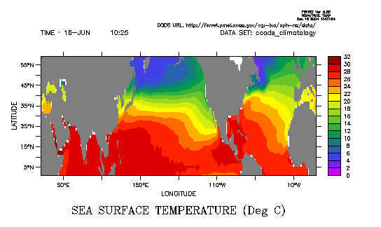
(Under linux only) var[d=filename] failed if the filename starts with a digit. These files can now be opened correctly.

When the dataset is an OPeNDAP (DODS) file, the label containing its URL now shows the complete path. (Further work on this is anticipated to minimize crowding of the labels in the top margin of the plot.)
```
yes? SET DATA "http://www.ferret.noaa.gov/cgi-bin/nph-nc/data/coads_climatology.nc"
yes? SHADE/L=1 sst
```

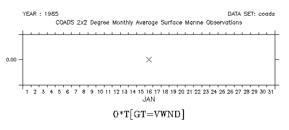
If the /HLMITS qualifier resulted in in a span containing just one coordinate point for a variable being plotted, we saw an error message. These plots can now be made.
```
yes? ! Show the location of the time coordinate in January 1985
yes? USE coads
yes? PLOT/SYM/SIZ=0.3/HLIM="1-jan-1985": "1-feb-1985" 0*t[GT=vwnd]
```

Illegal value of 0 in a stride crashed Ferret. This now gives an error message:
```
yes? LIST/I=1:300:0 var
```

Bug crashed Ferret when regridding with @NRST between two different calendar axes (e.g. Gregorian and Julian) for some time ranges. This is fixed.

Bug overlaying a polygon on a non-Gregorian time axis is fixed.

yes? USE coads_climatology
yes? SET AXIS/CAL=JULIAN time
yes? PLOT/X=140W/Y=0 sst
yes? PLOT/OVER/VS/LINE=3 {400,900,900,400}, {25.5,25.5,26.5,25.5}
yes? POLY/OVER/PAL=green {400,900,900,400}, {25.5,25.5,26.5,25.5}

When the missing-data value is NaN, some list commands such as SHOW DATA/FULL caused Ferret to crash (linux only). This is fixed.