Ferret is a workstation-based visualization and analysis environment designed to meet the needs of physical scientists studying global ocean/climate interactions. The scientist working with Ferret is provided with a highly-automated, flexible, end-to-end environment in which he/she can probe large and complex gridded data sets, such as model outputs and observational data products, with little or no assistance from computer professionals. The design of Ferret has emphasized close integration of graphics, analysis, and data management. Ferret provides well-proven scientific graphics styles, such as contours, scatter plots, and vector diagrams, and the ability to define new variables as mathematical expressions involving data base variables. Analysis is augmented by regridding capabilities and boolean operators to perform calculations over arbitrary regions. Ferret's data management is based on a simple, adaptable data model incorporated into standardized, self-describing, direct-access files.
Ferret is a workstation-based visualization and analysis environment designed to meet the needs of physical scientists studying global ocean-climate interactions. Ferret was developed as an adjunct to the numerical modeling studies of the Thermal Modeling and Analysis Project (NOAA/TMAP); work on the program began in 1985 when workstations were just becoming available. Ferret was created in the belief that unifying data management, analysis, and visualization and placing them directly in the hands of scientists would lead to new levels of productivity. The success of the approach has been evident in the growing use of Ferret since it was made publicly available in 1991; Ferret is now installed in approximately 75 laboratories and universities in at least 12 countries with the community of users growing steadily. With the imminent release of the point and click interface presented in this paper we expect growth in the use of Ferret to accelerate.
A recent report on the use of scientific visualization within the NASA EOSDIS community (Botts, 1993) pointed out that the use of visualization tools by earth scientists lags well behind the state of visualization technology. Key among the causes that were identified are
The report also points out that advanced visualization environments tend, unfortunately, to ignore the power and simplicity of simple graphical forms such as line plots and contours. The design of Ferret has emphasized tried-and-proven solutions: conventional scientific graphics, analysis based on user-definable variables built with simple mathematical tools, and a simple data model well-integrated into fundamental data base and file concepts.
A number of popular applications, notably Matlab (MathWorks, 1992) and IDL (Research Systems, 1993), have successfully integrated analysis with visualization and provided flexibility. However, they are "low level" environments wherein the user must be an adept programmer. The data base and file management tools provided are rudimentary. Other tools such as AVS (AVS, 1992) and Khoros (Khoral Research) have created higher-level environments but they are systems of great complexity — difficult to master and difficult to get data into. These tools are often better suited to dedicated computer professionals than to ocean scientists. The goal of Ferret is to bridge these gaps — to remain high level, flexible, and simple enough to be placed directly in the hands of a scientist whose concentration is focussed on scientific questions rather than on computer issues.
Depending upon individual taste and the nature of the visualization/analysis task a user may choose among three distinct interfaces to Ferret — a "point and click" X-windows interface, which is "friendly" for browsing and exploration; a World Wide Web interface, which enables remote users to access data via Ferret over an Internet connection; and a command line interface, which is best suited to complex data manipulations. In this section we will present the two graphical interfaces. The command line interface will be presented following an overview of Ferret's capabilities.
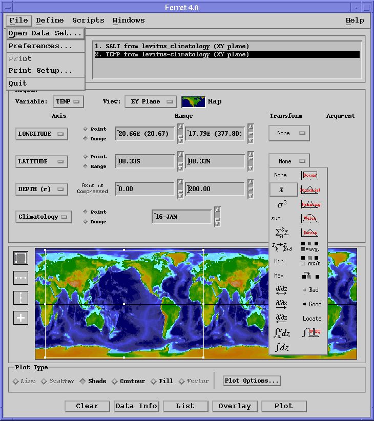
Figure 1. Main windows of Motif interface to Ferret.
The X-windows interface, built upon the Motif tool kit, is a recent addition to Ferret (in beta testing at the time of this writing). It makes Ferret easily accessible to first-time or infrequent users. Bringing up Ferret leads to a display similar to figure 1 with the region and variable fields empty. A session typically begins by selecting Open Data Set under the File menu; Ferret presents a scrollable list of data sets from which to choose. The list is culled from available files in directories distributed across a local area network; the list of directories is defined when Ferret is invoked. Seldom does the user seldom need to navigate directory trees to locate a data set.
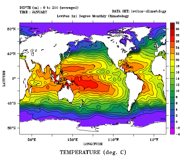
Figure 2. Typical Ferret browsing image.
Upon selection of a data set Ferret presents a map for browsing,
menus to choose variables of interest, and tools for navigating among
the dimensions of the data set. Other tools provide metadata —
information about the variables in the data set. The user can specify
the view of the variable (lat-long, long-depth, lat-time, etc.) and
the type of output desired (listing, line plot, contour map, etc.).
Frequently the user wishes to evaluate some sort of transformation on
the variable (smoothing, averaging, statistical summary, etc.); the
menu of transformations shown in figure 1 can be applied to any axis
of the variable. Figure 1
shows how the interface would be used to
produce

Figure 3. Text command input in the Ferret Motif interface.
The Motif interface is implemented quasi-independently from Ferret. It communicates with Ferret using a private query language (to determine the state of Ferret) and by issuing human- readable Ferret command strings. In principle the interface could be an application running on a separate machine from Ferret, though the authors have not seen sufficient utility in this to motivate development of the capability. The commands issued to Ferret are logged in a Script Manager window where the user can optionally edit them, resubmit them, and type in new commands [figure 3]. The Script Manager makes it possible to seamlessly blend the generality of a command line with the friendliness of a the point and click framework.
The Internet and the World Wide Web (WWW), augmented by pioneering and widely available applications such as Mosaic (NCSA, 1993) and Netscape (Netscape, 1994), have the power to radically enhance how ocean scientists share data in the future. However, significant barriers must be overcome: oceanographic data sets are frequently too large to be efficiently transferred over the Internet. Once transferred, data files suffer from incompatible, discipline-specific formats that make the files difficult to ingest into applications.
With the prototype WWW interface to Ferret we have created a data server with features that break through these barriers. The difficulties of overly-large data sets are minimized by interactive browsing capabilities; when a scientist can adequately browse data he/she need only download the region and variables of specific interest. In the case of multi-variate, gridded data, such subsets will often be orders of magnitude smaller than the full data set. The difficulties of incompatible file formats are minimized by providing the data in a user- selectable format. These custom-specified, formatted data files, like the graphics, must be created by Ferret in real time. The prototype of this interface is available on-line at http://www.ferret.noaa.gov/fbin/climate_server. This version makes accessible only a subset of Ferret's visualization capabilities and none of its analysis functions. Future versions will extend this functionality.

Figure 4. Main window of the World Wide Web interfave to Ferret.
Figure 4 shows the prototype Ferret WWW interface as it appears in the Mosaic program. Like the Motif interface, it provides controls to choose a data set, select a variable of interest, and navigate among the dimensions of the variable. The user can click on controls to request graphical products, listings (spreadsheets), or formatted files.
The Ferret WWW interface is created with the hypertext markup language (HTML), the language of WWW. HTML provides limited tools for graphical input with a feature called a "form". Most interfaces based on HTML forms have a static look-and-feel, a result of the stateless nature of the underlying network protocols. Statelessness means that the server has no "memory" of a (remote) users previous interactions; opening a data set, for example, is not a valid discrete request to make of a stateless server because it implies a state change from "file closed" to "file open" in the server.
With the Ferret WWW interface we have striven to create an interface that has a feel typical of more advanced graphical applications. Key to this has been the caching of state information within the client application through the use of "hidden input tags". A user can choose (open) a data set; select a viewing geometry; zoom into the region of interest; enter point locations normal to the axes of the view; and request graphical results or data downloaded in a choice of formats. A record of the user's actions is retained in the Ferret WWW interface as hidden input so that the interface "remembers" which data set has been opened and resends this information to the (stateless) server in subsequent commands.
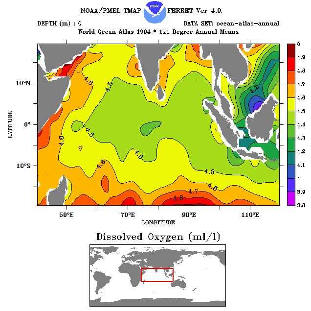
Figure 5a. Ferret WWW browse image in latitude-longitude plane
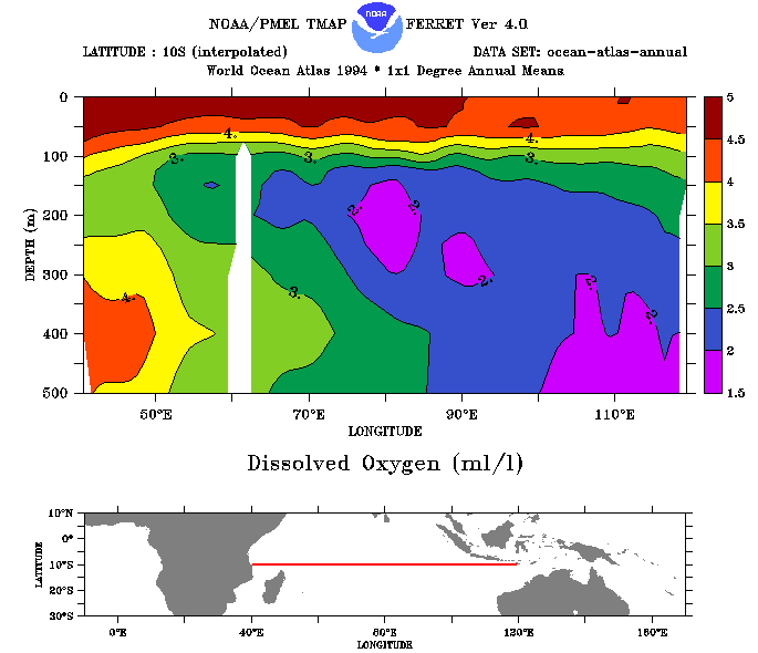
Figure 5b. Ferret WWW browse image in longitude-depth plane
The Ferret WWW server produces graphics and data files on-the-fly so the user has virtually limitless ability to request custom views of the data. For example, a user who wishes to investigate oxygen concentration in the ocean might select the variable DISSOLVED OXYGEN from the World Ocean Atlas 1994 (Levitus et al., 1994). Using the zoom interface he/she could select, say, a region in the Indian Ocean and obtain figure 5a. By changing views and zooming in depth the user might obtain a vertical profile plot such as figure 5b. The same data can be perused as numbers be requesting "spreadsheet" output [figure 6]. If the data is needed for local analysis Ferret will supply it as a self-documenting ASCII file or in netCDF format, suitable for Ferret or other applications running on the local host computer.
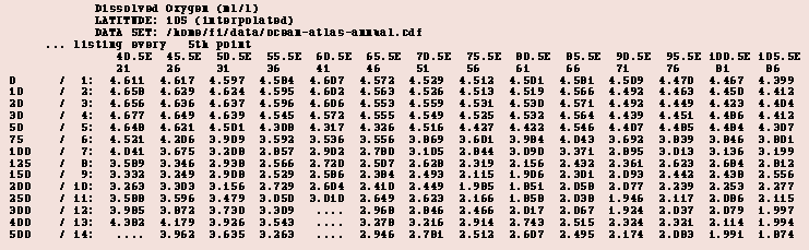
Figure 6. "Spreadsheet" output from Ferret WWW interface.
The interactions between the WWW server software and the Ferret program are handled as follows [figure 7]: when the server receives a request for data or graphics it first checks a cache of such files to see if the result has already been computed. If not, the server invokes Ferret as a command line program, redirecting I/O to communicate with Ferret via Unix pipes. The server then sends ASCII commands to Ferret — typically sending just a GO command to run a script. Arguments to the GO command usually include the name of the data set, the variable name, and the limits of the region requested. The script file contains the sophistication necessary to guide Ferret in producing appropriately laid out graphics, including reference maps [figure 5].

Figure 7. Schematic of WWW Ferret server.
Ferret is an end-to-end environment that integrates three disciplines: data base management, visualization, and analysis. In the development of Ferret there have inevitably been trade-offs between the advantages of sophisticated solutions to problems within these disciplines, and the need for integration, usually implying simplicity. The Ferret developers have, in almost all cases, opted for simplicity and integration. Since Ferret is the by-product of oceanographic research activities undertaken by a small group, limitations of programmer resources have necessitated this approach. The approach has, however, also contributed to the long term success of the program.
Ferret graphics are based on the interactive application, PLOT+ (Denbo, 1987), which is embedded within it. PLOT+ provides a range of 1-dimensional and 2-dimensional graphics types: contour plots (outline and color filled), rasters (images), line plots, and scatter plots, as well as mesh diagrams for limited 3-dimensional visualization. Ferret has an "intelligent" connection to the self-describing data sets it uses so all graphics are fully and unambiguously labeled by default; the design goal of Ferret, in this respect, has been that if a scientist distributes Ferret graphics to colleagues they should be able to reproduce the results from the default information which labels the plots. Ferret and PLOT+ also provide options for customizing layout, labels, color palettes, etc. To create animations, Ferret saves raster outputs in HDF (NCSA, 1994) files; excellent public domain packages such as XDataSlices and XCollage (NCSA, 1990) are available to animate these files.
Ferret's analysis strategy begins with a collection of basic transformations ("filters"), including derivatives, integrals, statistics, missing-value fillers, smoothers, value locators, and others, that may be applied symmetrically along any axis of a variable. Transformed and untransformed variables may then be combined in mathematical expressions using a familiar algebra of operators (+,- ,/,...) and functions (SIN, MAX, INT,...). New variables may be defined from old — complex analyses proceed as a hierarchy of variable definitions (see Sample Analysis).
One particularly powerful transformation computes an "integrating kernel" which locates a value or condition within a multi-dimensional field. By integrating the product of this kernel function times other fields the user may view results on arbitrary iso-surfaces. A simple example would be to view salinity on the 20-degree isotherm; a complex example might involve defining, as a surface, the depth at which two variables are in equilibrium.
Analysis frequently involves calculations applied over arbitrarily-shaped regions. For example, a physical oceanographer studying wind bursts may wish to focus on the rate of sea surface temperature (SST) change only in those regions which are experiencing easterly winds. Ferret provides this functionality through an IF-THEN-ELSE syntax which may be used in any mathematical expression. In our example, the scientist might define a new variable, EAST_DSSTDT, that is the time derivative of SST only IF the winds are easterly (ELSE the points are excluded from the calculation). Regions defined by this means need not be static — they can change shape and size as a function of time. In our example the scientist could obtain the time history of averaged d/dt(SST) within regions experiencing easterly winds simply by requesting a time series of the variable EAST_DSSTDT averaged in X and Y.
A special source of flexibility in Ferret is the ability to unify data sets that are defined on differing grids. A grid, in the sense in which we use the term within Ferret, is a collection of N axes forming an outer product of N-tuples. An axis is simply a monotonically ordered set of discrete points. The classes of data used in climate research vary widely in their grid structures: numerical model variables may be on staggered grids with irregularly-spaced points; gridded climatologies are built upon many different spatial and temporal resolutions and may have grids of latitude-longitude, lat-long-depth, lat-long-time, or other geometries; observational data may include time series, vertical profiles, and scattered point observations. The Ferret user simply chooses the desired destination grid and requests that variables be presented on this grid using a choice of regridding techniques. New axes and grids can also be defined. With the flexibility afforded by regridding Ferret can merge data from a variety of sources into a single calculation for analysis and visualization.
The simple data model that unifies all aspects of Ferret is the "gridded variable", a data object that combines a multi-dimensional raster with the coordinate locations of its underlying grid. The data types that climate researchers most commonly encounter map readily onto this structure (model outputs, binned climatologies, time series, profiles, ...). Other data types can be mapped onto gridded variables in various ways. For example, a sigma coordinate system (layered model) might be represented with the vertical axis coordinates as index values, alone; the true vertical positions are computable as the vertical integral of layer thickness. Scattered point observations, another example, may be viewed as collections of one-dimensional gridded variables: coordinates and values. Where the mapping of the data onto the gridded variable model becomes complex, the sophistication required of the user grows greater, but the authors have seldom encountered data models that they were unable to work with.
Ferret supports a number of data formats: the most commonly used is netCDF (Rew, 1990). NetCDF is a self-describing, direct access format and widely used within the oceanographic community. The gridded variable data model maps readily onto the structures provided by netCDF. Ferret can also ingest ASCII and binary floating point files; variable names, units, and grid coordinates are defined on-the-fly by the user. Output files can be ASCII, binary, or netCDF, so Ferret can also function as a file format converter.
Memory management within Ferret is optimized for very large data sets. As the user opens data sets, defines new and transformed variables, and specifies regions in space and time Ferret does not access data. It is only when a result is requested — a plot, listing, or summary statistic — that data I/O takes place. By deferring I/O, Ferret "knows" the minimum data required for the calculation and reads only that subset from the direct access files. (Data are cached in memory to enhance the performance of subsequent commands.) This strategy also permits Ferret to perform calculations of size far exceeding the apparent limits of computer memory. For example, calculating a time-series of model-produced ocean temperature averaged in three dimensions may require hundreds of megabytes of component data; Ferret will transparently break such a calculation into manageable fragments to compute the result.
Ferret's command line interface works in any ANSI terminal environment, providing recall of past commands and command line editing with the cursor arrow keys. The Ferret command language consists of 20 commands (PLOT, CONTOUR, LIST, LET, ...) and a variety of subcommands and qualifiers. The user can query Ferret for the command names with the command SHOW COMMANDS; the Ferret Users' Guide provides detailed descriptions.
The user refers to variables by name ("temp", "salt", "taux", ...) and specifies regions of interest using a mixture of world coordinates and index values as needed: X, Y, Z, and T for axis positions specified as world coordinates, and I, J, K, and L to specify indices. The region information may apply to an entire command (slash-separated) or to a single variable (using square brackets). Examples of Ferret commands which specify regions in various ways are
Item (i) sets "15-JAN-1982" as the default date of interest, (ii) produces a vector arrow plot of U and V velocity components at 100m depth, and (iii) produces a contour plot of the variable named "TEMP" at K=1, the first vertical index.
The user may request that transformations such as averaging or differentiating be applied to a variable along a particular axis. To do so he/she modifies the region specifier with an "@" sign followed by the transformation name. For example, the command CONTOUR TEMP[Z=0m:500m@AVE] is a request to contour the variable TEMP (temperature) averaged from 0 to 500 meters in depth.
The user may combine variables to form algebraic expressions. Optionally, he/she may define new variables from these expressions using the LET command. For example, the command CONTOUR TEMP[Z=100] - TEMP[Z=0:500@AVE] would contour the temperature anomaly at 100 meters depth relative to the temperature averaged from the surface to 500 meters. The command LET HEAT_FLUX = WIND_SPEED * (SST - AIR_TEMP) might be used to define the new variable "heat_flux", a sensible heat flux calculation.
Ferret's command language is also a scripting language; groups of commands may be saved in a file (script) and executed with the GO command, optionally passing arguments to the script. A collection of commonly used scripts is provided with Ferret. For example, GO basemap X=10W:170E Y=30S:10N produces the reference map shown in figure 5b.
The following calculation illustrates the style with which a Ferret user may probe data sets. In this example our goal is to characterize the seasonal cycle of heat content within the mixed layer of the Pacific Ocean at longitude 155°W (the Hawaiian Islands). We will use the data-rich COADS sea surface observation data set (Slutz et al., 1985; Woodruff et al., 1987) to obtain monthly, gridded sea surface temperatures. We will estimate the depth of the mixed layer from the vertical temperature structure of the multi-layer Levitus climatology (Levitus, 1982). Combining the two results, we will obtain an estimate of the heat content within the mixed layer of the Pacific Ocean in one particular month. We will then examine the value of the mixed layer heat at longitude 155°W and will extend this result to the annual cycle.
We begin the exploration with basic browsing — either with the mouse or the command line interface. We select the data sets we wish to use, monthly climatologies of Levitus and COADS data. Figure 2 is a typical browsing output, a labeled contour plot of Levitus ocean temperature, vertically averaged from the surface to 200 meters in January, with an overlaid land outline.
The Levitus climatology is 1 by 1 degree in horizontal resolution with TEMP (temperature in °C) available at 19 unevenly-spaced layers. We will use Levitus's technique for computing the mixed layer thickness as the depth at which temperature has decreased by 0.5 °C from its surface value. To do so we will subtract the vertical temperature field from the surface temperature; the depth of 0.5 in the resulting field (TEMP0) will give us the Levitus mixed layer thickness, ZMIX. The Ferret transformation LOC, that locates (interpolates) the first occurrence of a given constant along an axis, is the key in the following definitions:
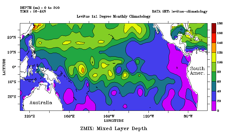
Figure 8. Sample analysis: mixed layer depth from Levitus.
(The optional inclusion of Z=0:200 confines the search for the constant 0.5 to a limited depth range to improve performance.) Figure 8 shows the resulting field as a filled contour plot with land outlines.
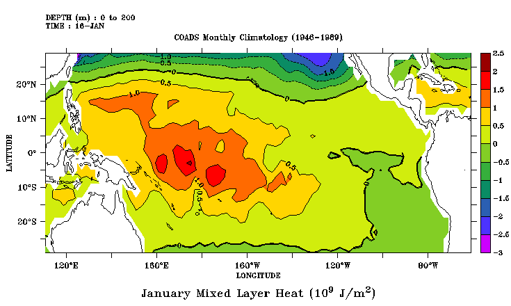
Figure 9. Sample analysis: mixed layer heat content
The COADS data set, which includes the SST values we will use in this calculation, is 2x2 degrees in horizontal resolution. In the interest of simplicity we will assume a constant value of Cp =3900 Joules/kg-°K and base heat content on the SST anomaly from a single climatological background value for the region, SSTAVE, defined as the COADS SST averaged both horizontally and in time. Since the COADS SST is defined on a 2 by 2 degree grid, whereas ZMIX, based on temperature from the Levitus data set, is defined on a 1 by 1 degree grid, regridding is required. The syntax G=SST, below, performs the regridding to the grid of COADS SST using the default bi-linear interpolation. These are the exact commands that produced figure 9 (superscripts were used to demonstrate the graphic capability; their precise syntax is not presented):
J/m)"
QMIX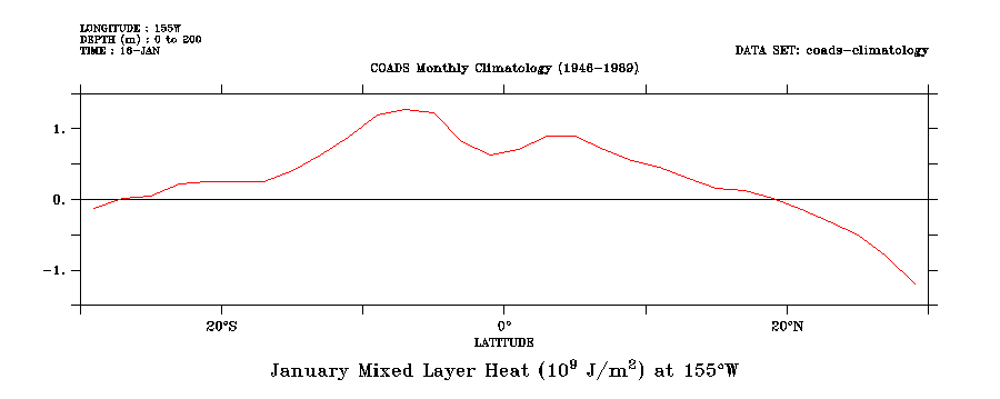
Figure 10. Sample analysis: mixed layer heat content along 155°W.
Now we wish to focus our attention on a meridional section along longitude 155°W. We browse QMIX to obtain figure 10, a plot of the heat content along longitude 155°W.
Since our goal is to "characterize" the heat content we need to generalize the result we have obtained for January to the annual cycle. We could create an animation of successive months using a REPEAT loop over time, optionally with interpolated frames. However, for this illustrative example, we will instead generalize the one-dimensional plot of figure 10 to a two-dimensional Hovmoller plot of latitude and time. We use basic browsing controls to specify a time span of two years (two years provides a clearer view of the annual cycle than does a single year). In figure 11 we have, in addition, smoothed the result with a 5 point running mean (boxcar) smoother in latitude and a 3 point smoother in time. Note that the documentation regarding smoothing in the title of the figure was produced by Ferret's automatic labeling facility.
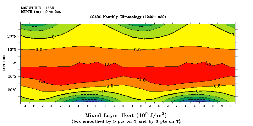
Figure 11. Sample analysis: annual cycle of mixed heat content at 155°W.
Figure 11 illustrates the seasonal cycle of mixed layer heat content. Notice the expected out of phase behavior between the Northern and Southern hemispheres. Also note the asymmetry between the north and south within the Tropics which invites further investigation.
In this paper we have presented an overview of the program Ferret: its interfaces, its capabilities, and examples that illustrate the style of its use. We have shown how a simple data model, the multi-dimensional gridded variable, has been used to integrate two-dimensional scientific graphics, analysis based on axis-symmetric transformations and user-created hierarchies of variable definitions, and a simple data base strategy of direct-access, self-describing files. With this integration we have created a high-level, yet simple-to-use visualization environment suitable for direct usage by scientists, rather than by computer specialists.
Ferret is still evolving and growing as resources become available. Future work will focus on the maturation of the graphical user interfaces, bringing more of Ferret's analytical capabilities under point-and-click control through both Motif and the World Wide Web. Analytical capabilities will be expanded to include frequency domain tools and greater facility with objective and optimal interpolation for improved handling of observational data. Enhancements to the data base schema will support multi-dimensional arrays of netCDF files as virtual data sets, permitting Ferret to handle data sets of terabyte size.
Ferret is available at no charge via anonymous ftp at abyss.pmel.noaa.gov [192.68.161.20]. Installation is straightforward; Ferret is supplied in binary for Sun (SunOS, Solaris), DEC (OSF, Ultrix), SGI (Irix), and IBM (AIX), with a port to HP underway at the time of this writing. Examples, tutorials, and a 200 page Users' Guide are provided.
We would like to acknowledge the generous and future-looking assistance of the Laboratory directorate at PMEL; the direct funding of graphical interfaces that has been supplied by the NOAA/ESDIM program; and the members of the NOAA/EPOCS council for their support during the early development of Ferret. Special personal thanks go to Jim Holbrook, who has opened doors and provided encouragement at every step.
AVS, 1992: AVS Users' Guide, Advanced Visual Systems, Inc., 300 Fifth Ave., Waltham, MA 02154, support@avs.com
Botts, M.E., 1993: The State of Scientific Visualization with Regard to the NASA EOS Mission to Planet Earth, A Report to NASA Headquarters. Earth System Science Laboratory, The University of Alabama in Huntsville, AL 35899 (botts@stromboli.atmos.uah.edu).
Denbo, D.W., 1987: PLOT PLUS Scientific Graphics System Users Guide, Plot Plus Graphics, P.O. Box 4, Sequim, Washington
Hankin, S., J. Davison, K. O'Brien, and D.E. Harrison, 1992: FERRET A computer visualization and analysis tool for gridded data. NOAA Data Report ERL PMEL-38, 164 pp.
Khoral Research, Inc.: 6001 Indian School Rd. NE, Suite 200, Albuquerque NM 87100, khoros-request@khoros.unm.edu
Levitus, S., 1982: Climatological Atlas of the World Ocean, NOAA/ERL GFDL Professional Paper 13, Princeton, N.J., 173 pp. (NTIS PB83-184093).
Levitus, S. et al., 1994: World Ocean Atlas 1994, 4 volumes, Washington, D.C., NOAA/NESDIS/NODC.
The MathWorks, Inc., 1992: MATLAB Users' Guide, 24 Prime Park Way, Natick, MA, info@mathworks.com
Netscape, 1994: Netscape Navigator Version 1.0, Netscape Communications Corporation, info@netscape.com
NCSA, 1990: NCSA X Image for the X Window System, Version 1.0. National Center for Supercomputing Applications, University of Illinois at Urbana-Champaign.
NCSA, 1993: NCSA Mosaic for the X Window System, mosaic@ncsa.uiuc.edu.
NCSA, 1994: The HDF Reference Manual , Version 3.3, (http://hdf.ncsa.uiuc.edu:8001/refman/refmanual.html)
Research Systems, Inc., 1993: IDL Reference Guide, Version 3.1, RSI, 777 29th St., Boulder CO 80303.
Rew, R.K., and G.P. Davis, 1990: The Unidata netCDF: Software for scientific data access. Sixth International Conference on Interactive Information and Processing Systems for Meteorology, Oceanography and Hydrology, Feb 5–9, 1990, Anaheim, CA.
Slutz, R.J. et al., 1985: Comprehensive Ocean-Atmosphere Data Set; Release 1. NOAA/ERL Climate Research Program, Boulder, CO, 268 pp. (NTIS PB86-105723).
Woodruff, S.D. et al., 1987: A Comprehensive Ocean-Atmosphere Data Set, Bull. Amer. Meteor. Soc., 68, 1239–1248.