Background
All the details for using the trajectory, profile and point (timeseries) data set capabilites available starting with v8.2. N.B. To use LAS with ERDDAP discrete geometry data you must arrange for your data to include two columns that specify the longitude of the observation. In the first such column, the values should range from -180 to 180 in the second column (called lon360) re-normalize the values so they range from 0 to 360. N.B. If you want to use the "season" selection widget you must introduce a column into your data set which identifies the month in which the observation was taken with one of the following 12 strings, "Jan", "Feb", "Mar", "Apr", "May", "Jun", "Jul", "Aug", "Sep", "Oct", "Nov", or "Dec".
Data organized in various discrete geometries such as time along a path which is being served by ERDDAP can be configured into LAS and can take advantage of many special user interface elements and plot types.
This is an example of a plot of trajectories on a map.
The path of the platform is colored by the value of the parameter being displayed.
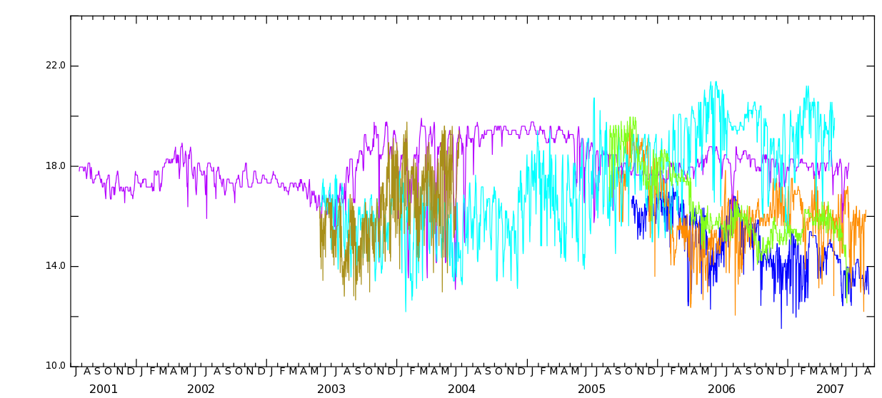
Point data, with or without a z-axis can also be configured into LAS and plotted. The map plot for these data places a disk at the location of the observation and colors segments of the disk according to the value of the parameter. For profile data, the segments around the disk show the value of the parameter long the vertical axis and for time series data the segments around the disk change with time.
In addition to the custom plot types available, the new capabilities for handling discrete geo-metries in LAS include custom constraint widgets that allow users to select sub-sets of the features based on metadata variables from the data set. The id, platform type, and the name of principal investigator are examples of the type of subsetting that might apply to discrete geometry data.
When data are ingested into ERDDAP certain metadata associated with a collection can be designated as a “sub-set” variable. This means that some sub-set of the features in the collection are associated with a single value of the sub-set variable. In some instances like the ID, the mapping is one-to-one, but in many other cases like the name of the ship taking the observations the mapping can be one value to many individual features.
Each of these two types of sub-set variables is represented by its own widget in the user interface.
The image at below shows the “Select” widget which will select an individual trajectory using a sub-set variable, the trajectory ID, that has a one-to-one mapping to the data. The “by Cruise Metadata” widget which can be opened by clicking on the title will expose a similar widget which contains variables, like the ship name, which are mapped to the data as one-to-many. Of course, in either widget more than one value can be selected and applied to an LAS product.
Configuring the ERDDAP Access to the Collection
To begin, we developed a tool you can use to create a configuration. It's possible that the configuration will not be complete and you will have to edit the resulting file. But, editing the file should be much easier than starting from scratch. All of the details about the resulting configuration are given below.
To build a sample configuration for each of the discrete geometry types we support, run the following commands:
./bin/addDiscrete.sh -u http://upwell.pfeg.noaa.gov/erddap/tabledap -i NOAAShipTrackWTEC (A trajectory data set)
./bin/addDiscrete.sh -u http://coastwatch.pfeg.noaa.gov/erddap/tabledap -i erdCinpKfmT (A time series of SST at various stations)
./bin/addDiscrete.sh -u http://ferret.pmel.noaa.gov/erddap/tabledap -i profiles_b1fc_d6f5_b401 (profile)
Where the -u argument is the base URL of the tabledap section of the ERDDAP server and the -i argument is the ID of the data set that contains the discrete geometry data. Each command will create a file called las_from_scanerrdap.xml.
The software will attempt to automatically find and configure the “sub-set” variables, the variables that represent latitude, longitude, and time and the dependent variables. It will also make special configuration properties for a table of property-property plot thumbnails and for the property-property viewer.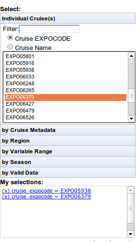
Finally, for large data sets you might want set up a display_lo and display_hi value. When the data set is selected in the UI, the time widget will be set to the display_lo and display_hi values. Choosing a small interval will prevent the UI from automatically requesting a large amount of data when the data set is first selected.The final result of the edit, will look something like this:
 <time-OSMCV4_DUO_SURFACE_TRAJECTORY type="t" units="day" display_lo="01-APR-2013" display_hi="02-APR-2013">
 <arange start="2013-04-01 00:00:00" size="30" step="1" />
 </time-OSMCV4_DUO_SURFACE_TRAJECTORY>
N.B. the "Ferret" format of the time specification in the display_lo and display_hi attributes.
Specify use of the discrete geometry UI
Here are the details about the configuration for a collection of discrete geometry files being served by ERDDAP so that they can be used in LAS and take advantage of the special features for discrete geometry data. All of this will be done for you automatically the addDiscrete.sh software.
First you must add the following <ui> property which will load up the special UI features and LAS products whenever this data set is selected.
<trajectory_dataset name="My Trajectory Data” url="http://dunkel.pmel.noaa.gov:8660/erddap/tabledap/">
 <properties>
 <ui>
 <default>file:ui.xml#Trajectories</default>
 </ui>

...
Configure Access to the Data Set
Then there is a block of properties to described the data in ERDDAP. This block of XML appears as part of the definition of the data set under the <properties> element within an element called <tabledap_access>.
<socat name="Surface Ocean CO‚ÇÇ Atlas" url="http://my.erddapserver.org/erddap/tabledap/">
 <properties>
 <ui>
 <default>file:ui.xml#Trajectories</default>
 </ui>
 <tabledap_access>
 <server>ERD TableDAP</server>
 <id>datasetID_04fd_e972_77c8</id>
 <title>My Trajectory Data</title>
 <longitude>longitude</longitude>
 <lon_domain>-180:180</lon_domain>
 <latitude>latitude</latitude>
 <time>time</time>
 <time_units>sec since 1970-01-01T00:00:00Z</time_units>
 <time_type>double</time_type>
 <trajectory_id>cruise_expocode</trajectory_id>
 <orderby>cruise_expocode,time</orderby>
 <dummy>temperature</dummy>
 </tabledap_access
There are about a dozen elements of information that you must fill out about your server
After you have installed ERDDAP and configured you discrete geomertry data into the server, you can find an unique ID for the data set on the “tabledap” page of the ERDDAP server. This URL is also the URL that you should enter as the URL for the data set (set to http://my.erddapserver.org/erddap/tabledap in this example). The ID is the last column of the display labeled Dataset ID.
Within the trajectory data set there must be columns that represent the time, longitude and latitude of each observation. These columns must be identified by name in the <time>, <longitude> and <latitude> elements respectively. In our example, these variables are called time, longitude and latitude respectively. You can find the names of these variables by looking at the data display for this data set in ERDDAP. The URL with the base URL you defined in the url attribute of the data set definition followed by the ERDDAP Dataset ID. (http://my.erddapserver.org/erddap/tabledap/datasetid_04fd_e972_77c8 in our example).
The <lon_domain> give the range of the longitude values found in the data set. This will always be set to -180 to 180 (see the note in bold at the top of the document).
The <time_units> and the <time_type> give us information about how to translate back and forth between the number stored the ERDDAP time column and a standard calendar string like 1962-03-06 02:24:00. The time units are express as [Well Known Unit] since [DATE TIME STRING] (sec since 1970-01-1-T00:00:00Z in our example). And the values are of type double which is necessary to have enough precision to store the seconds since midnight 1970-01-01.
One very important bit of information that must be specified is the variable that contains the ID for the data set. When working with discrete geometry data, there is at least one variable whose value is constant for all of the times and locations that constitute a single feature. This variable is used for organizing the data into a netCDF CF DSG file and for the user interface element that allows users to select an entire feature. For example, when looking at the data display for a tabledap trajectory data set, the trajectory_id variable is easy to identify by looking at the attributes at the bottom of the page and find the variable with the cf_role attribute of “trajectory_id”. For example:
Attributes {
s {
cruise_expocode {
String cf_role "trajectory_id";
String long_name "EXPO Code";
}
In this case, the variable named cruise_expocode plays the role of the trajectory_id for this data set.Similarly, the id variable for profile data will have a cf_role of profile_id and a timeseries point will have a variable with a cf_role marked as timeseries_id.
Additional configuration elements must be specified to work with a discrete geometry data set in LAS. For some queries LAS wants to make it is only interested in the latitude, longitude and time variables, but ERDDAP expects at least one data variable to be present in each request. Pick one of the data variables from the data set and put its name in the <dummy> element. We used temperature in this example.
You can also sort the the resulting features. By default they are sorted by id and time which is the order necessary make the plots work correctly. Ideally, the data come out sorted from ERDDAP because they were properly sorted when the data were loaded. We want the plots to work even if the data is not sorted so we ask for them to be sorted correctly in every request we make. But, if you want to use your LAS for quality control to look for unsorted data use <orderby>none</orderby> to explicitly stop LAS from requesting the data be sorted.
The LAS Dataset Configuration for Discrete Geometries
After setting up the access to the ERDDAP server, the next configuration step is to create the standard LAS dataset and variable configuration. The majority of this configuration is identical to the configuration for data defined on a grid, but the section below highlights some important differences.
First of all, independent variables like, latitude, longitude and time appear in a row of data along with their dependent variable counterparts. And it is sometimes interesting to make plots of an independent variable vs a dependent variable in the correlation viewer. In order to enable this capability, the independent variables must be defined not only in the axes and grid specification, but in the list of data set variables. For example:
<variables>
 <time grid_type="trajectory" units="sec since 1970-01-01T00:00:00Z" name="Time" url="#time">
 <link match="/lasdata/grids/socat_grid" /> </time> <latitude grid_type="trajectory" units="degN" name="Latitude" url="#latitude">
 <link match="/lasdata/grids/socat_grid" /> </latitude> <longitude grid_type="trajectory" units="degE" name="Longitude" url="#longitude">
 <link match="/lasdata/grids/socat_grid" />
 </longitude> <fCO2_recomputed grid_type="trajectory" units="uatm" name="fCO‚ÇÇ Recomputed" url="#fCO2_recomputed">
 <link match="/lasdata/grids/socat_grid" />
 </fCO2_recomputed>
 <cruise_expocode color_by="true" trajectory_id="true" grid_type="trajectory" subset_variable="true" units="text" name="Cruise EXPOCODE" url="#cruise_expocode">
 <link match="/lasdata/grids/socat_grid" />
 </cruise_expocode>
Note also that each of these variables is marked with the grid_type="trajectory" attribute. It is the presence of this attribute that triggers the loading of the special UI elements and operations when such a variable is selected. Similarly, grid_type="profile" and grid_type="timeseries" will be set for the other feature types currently supported.
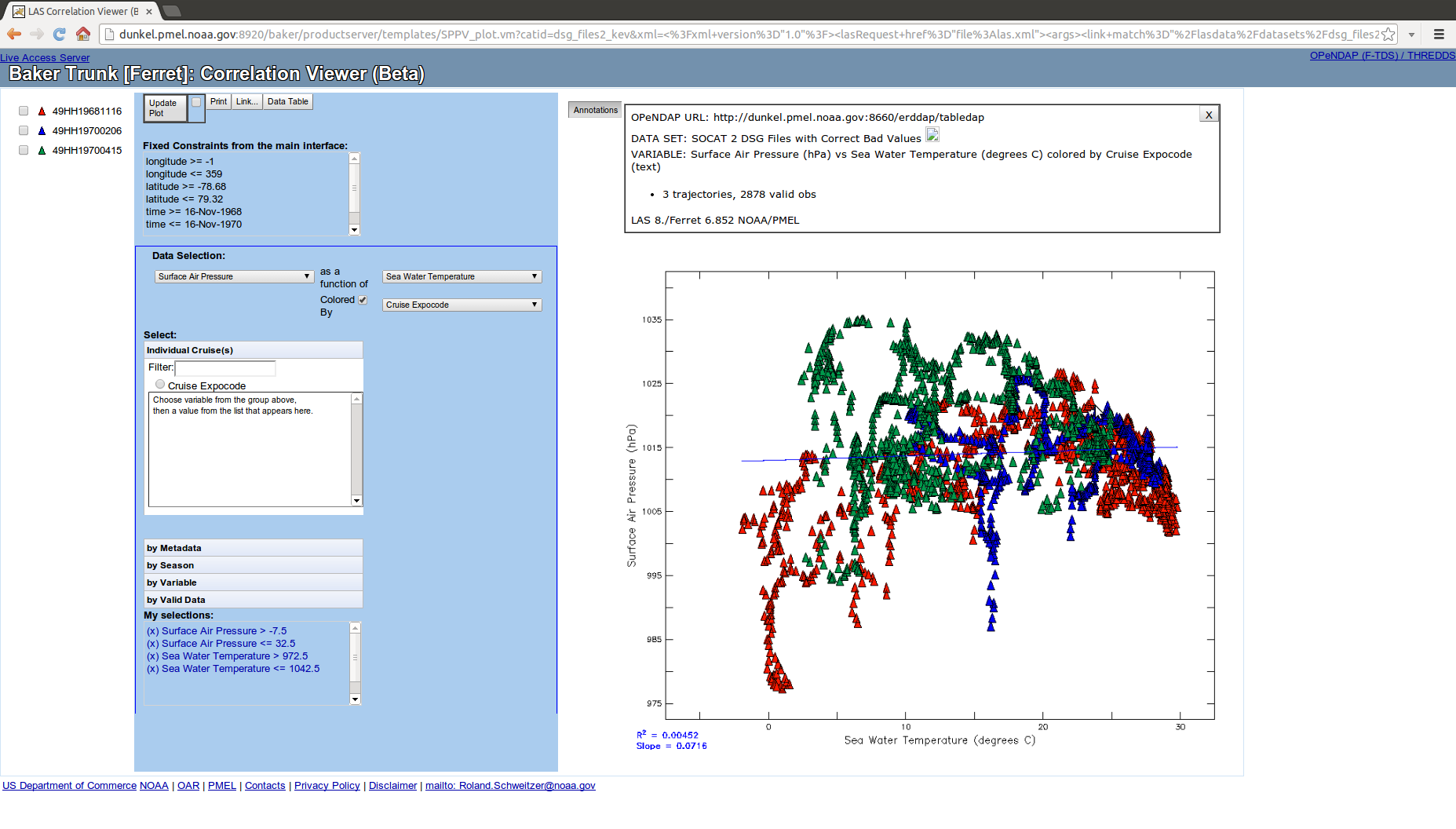
Also, take a close look at the cruise_expocode. Previously, we saw that this variable was identified in the properties as the trajectory ID. That fact should also be noted in the data set configuration with the trajectory_id="true" attribute. The <cruise_expocode> element also marked with the subset_variable="true" attribute. This prevents the variable from being listed as one of the variables for plotting on the map since the current backend scripts have not been enhanced to be figure out how to color the trajectories based on a variable that contains text as its value.Finally, the correlation viewer can plot the value of the property vs the value of the other where the each trajectory has a unique marker on the graph. To enable this capability, you must mark the variable with the color_by="true". This attribute is necessary for the special correlation plotting interface (Beta in v8.2) even though the variable is already identified as the trajectory ID.
To make exploration of the data with the property-property plot viewer work as fast as possible, the set of constraints active when the viewer starts will remain active through out the session. And all of the data which can be used in the session is extracted from ERDDAP once at the beginning. The names of the variables that can be used in the property-property viewer are defined in the configuration by the <all_variables> element.
Configure the UI Widgets
As discussed in the introduction, there are several new widgets that will appear in the LAS User Interface when a discrete geometry data set is selected. There is special configuration that is added to the LAS data set configuration to control the appearance and function of these widgets.
<constraints>
 <constraint_group type="selection" name="Individual Cruise(s)">
 <constraint name="Select By">
 <variable IDREF="cruise_expocode"/>
 <variable IDREF="cruise_name"/>
 <key>cruise_expocode</key>
 </constraint>
 </constraint_group>
 <constraint_group type="subset" name="by Cruise Metadata">
 <constraint widget="list">
 <variable IDREF="PIs"/>
 <key>PIs</key>
 </constraint>
 <constraint type="subset" widget="list">
 <variable IDREF="vessel_name"/>
 <key>vessel_name</key>
 </constraint>
 <constraint type="subset" widget="list">
 <variable IDREF="QC_flag"/>
 <key>QC_flag</key>
 </constraint>
 </constraint_group>
 <constraint_group type="subset" name="by Region">
 <constraint type="subset" widget="list">
 <variable IDREF="region_id"/>
 <key>region_id</key>
 </constraint>
 </constraint_group>
 <constraint_group type="season" name="by Season">
 <constraint widget="month">
 <variable IDREF="tmonth"/>
 <key>tmonth</key>
 </constraint>
 </constraint_group>
 <constraint_group type="variable" name="by Variable Range"/>
 <constraint_group type="valid" name="by Valid Data"/>
</constraints>
These blocks of XML get translated into User Interface widgets that let users constrain the data that is included in a particular product result. The first two function similarly with some subtle differences in the semantics of what features are selected.
The first group we will look at is will display a collection of variables which are mapped to the features in a data set one-to-one. The most obvious (and usually the only) such variable will be the ID. In this data set the trajectory ID is called cruise_expocode. As such we use the cruise_expocode as the “key” for all of the searches. Since the mapping for both variables is one-to-one, any other variable that maps one-to-one to the individual trajectories should map one-to-one to the trajectory id.
 <constraint_group type="selection" name="Individual Cruise(s)">
 <constraint name="Select By">
 <variable IDREF="cruise_expocode"/>
 <variable IDREF="cruise_name"/>
 <key>cruise_expocode</key>
 </constraint>
 </constraint_group>
When a data set adds this configuration the resulting widget will display the values of the variable to the user and when the search is made the it will use the corresponding “key” to make the search. In the case of the curise_expocde these two values are the same, in the case of the criuse_name, the value displayed to the user is different from the “key” value that is used for the search.
The second group functions the same, but selecting a value from this group might resulting the the selection of many features since the mapping for these variables can be one-to-many.
 <constraint_group type="subset" name="by Cruise Metadata">
 <constraint widget="list">
 <variable IDREF="PIs"/>
 <key>PIs</key>
 </constraint>
 <constraint type="subset" widget="list">
 <variable IDREF="vessel_name"/>
 <key>vessel_name</key>
 </constraint>
 <constraint type="subset" widget="list">
 <variable IDREF="QC_flag"/>
 <key>QC_flag</key>
 </constraint>
 </constraint_group>
In this case the variable and its key are the always the same.
These constraint group are is exactly the same as the “by Cruise Metadata” group above, but the semantics is special (a region of the earth) not a characteristic of the trajectory per se. So to be able to give the constraint widget its own title we simply add another constraint group with the same syntax as the previous with the title “by Region”.
 <constraint_group type="subset" name="by Region">
 <constraint type="subset" widget="list">
 <variable IDREF="region_id"/>
 <key>region_id</key>
 </constraint>
 </constraint_group>
The next group has as special semantics and a unique display for specifying the values. The data set has a column which identifies the month of the year in which the data point was collected. By specifying a constraint group of type “season” we the user interface will show the season constraint and the user can select any sequence of consecutive months (like DJF for example) to extract data collected during those months only. This
 <constraint_group type="season" name="by Season">
 <constraint widget="month">
 <variable IDREF="tmonth"/>
 <key>tmonth</key>
 </constraint>
 </constraint_group>
In the case of the region and season constraints the constraint applies to each data row, so it is possible that some of the selections made by applying such a constraint will result in only part of a trajectory being included in the LAS output product since the value changed part way through the cruise. This constraint will only work if you have a column in your data set which identifies the month in which the observation was taken using the appropriate string in the list: "Jan", "Feb", "Mar", "Apr", "May", "Jun", "Jul", "Aug", "Sep", "Oct", "Nov", or "Dec". We have a Ferret script that prepares this column for us and writes the result to a discrete geometry netCDF file before we import the data into ERDDAP. Using these strings we can do "OR" queries so that we can collect data from December, January and February. The sorting on the actual observation time keeps the trajectory geometry intact.
The next two are easy to include and easy to explain.
<constraint_group type="variable" name="by Variable Range"/>
Including a constraint group of this type will make a widget appear in your user interface which lists each variable (those variables that are not marked with the subset=”true” attribute in the configuration) and will allow the user to enter a high and low value. The next product created will constrain the data to be in the range. When a product is created, the actual range of the data being displayed will automatically be filled in on the widget to make it easier to know what to enter.
<constraint_group type="valid" name="by Valid Data"/>
Including this type of constraint group will cause a UI element to appear that will select variable where the data must be valid for the row to be included in the result. If for example want to see a plot of temperature vs salinity only where these is valid measurement for FCO2, choose FCO2 from the “by Valid Data” widget before requesting the product.
Configuration Properties for the Property-Property Viewer
In order to make exploring the data set with the property-property viewer as efficient as possible LAS will extract all of the data variables from ERDDAP instead of just the currently selected variable as it does with a map plot. This means that when a user wants to change one of the variables on the plot axis LAS can make the new plot without returning to ERDDAP to extract new data. Some data collections contain a massive number of variables, not all of which are suitable for use in the property-property viewer. The addDiscrete.sh software will create a list of variables and store the results in a property in the configuration.
<all_variables>windSpeed_kts,platformCourse,waterDepth_f,airTemperature,windSpeed_m_s,relativeHumidity,windDirection,platformSpeed_m_s,platformSpeed_kts,waterDepth_m,salinity,seaTemperature,airPressure</all_variables>
You can modify the list by adding new variables from the data set or by removing those variables which are not interesting for property-property plots. The variables are listed by their ERDDAP short name which is shown on the data page for the ERDDAP data set.
Configuration Properties for the Table of Thumbnail Plots
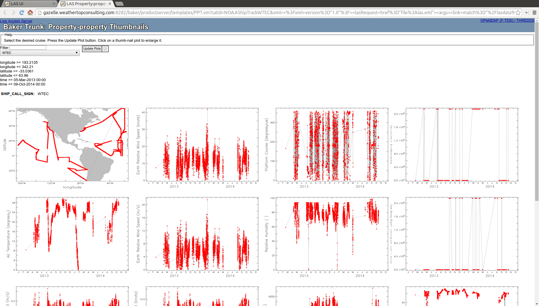
Another feature of LAS for trajectory data sets is a product that will produce a grid of thumbnail images of property-property plots. The thumbnails are live links to the property-property viewer so the user can easily explore any interesting plots on the the page. By default, addDiscrete.sh will configure LAS to create a thumbnail a plot of the latitude and longitude (just a simple track of the trajectory) and then to pair each data variable with time. For a profile, each variable will be paired with depth and for a timeseries each variable will be paired with time in addition to the latitude/longitude location plot. This is an area where the installer might want to consider adding other pairs to the configuration for such common plots as salinity vs temperature. All of the properties that control the thumbnail page are in the <thumbnail> property group.
The configuration of the plot pair are made by listing the LAS ID of the variables as shown below in the <variable_pairs> element.
<thumbnails>
 <variable_names>windSpeed_kts,platformCourse,waterDepth_f,airTemperature,windSpeed_m_s,relativeHumidity,windDirection,platformSpeed_m_s,platformSpeed_kts,waterDepth_m,salinity,seaTemperature,airPressure</variable_names>
 <variable_pairs>longitude-NOAAShipTrackWTEC,latitude-NOAAShipTrackWTEC
time-NOAAShipTrackWTEC,windSpeed_kts-NOAAShipTrackWTEC
time-NOAAShipTrackWTEC,platformCourse-NOAAShipTrackWTEC
time-NOAAShipTrackWTEC,waterDepth_f-NOAAShipTrackWTEC
time-NOAAShipTrackWTEC,airTemperature-NOAAShipTrackWTEC
time-NOAAShipTrackWTEC,windSpeed_m_s-NOAAShipTrackWTEC
time-NOAAShipTrackWTEC,relativeHumidity-NOAAShipTrackWTEC
time-NOAAShipTrackWTEC,windDirection-NOAAShipTrackWTEC
time-NOAAShipTrackWTEC,platformSpeed_m_s-NOAAShipTrackWTEC
time-NOAAShipTrackWTEC,platformSpeed_kts-NOAAShipTrackWTEC
time-NOAAShipTrackWTEC,waterDepth_m-NOAAShipTrackWTEC
time-NOAAShipTrackWTEC,salinity-NOAAShipTrackWTEC
time-NOAAShipTrackWTEC,seaTemperature-NOAAShipTrackWTEC
time-NOAAShipTrackWTEC,airPressure-NOAAShipTrackWTEC</variable_pairs>
 <metadata>ship_call_sign</metadata>
 </thumbnails>
At the top of the thumbnail page LAS will list some metadata to let the user know more about the feature being plotted. You can control which variables values are display at the top of the page by listing the ERDDAP variable names of the variables you want to include in the <metadata> element. In this case, the only metadata shown will be the trajectory ID, ship_call_sign which is added by default by addDiscrete.sh. An installer might want to add information like the principal investigator and the platform name to the list.
Finally, to make the plots most efficiently, LAS will extract all the variables necessary to do all of the plots when it's making the first plot. In order to do that, all the variables LAS needs for the thumbnails must be listed in the <variable_names> element.
Configuration Hints
If you have to build or fix the configuration by hand on the tabledap data page for a data set there is a block of netCDF-like metadata for each variable at the bottom of the page which is helpful for building the configuration.