A quick way to get to know Ferret is to run the tutorial provided with the distribution.
Run either "ferret" or "pyferret".
% ferret
yes? GO tutorial
If Ferret is not yet installed consult the chapter "Computing Environment" (The tutorial is also available on-line through Ferret's on-line demonstrations page.) The tutorial demonstrates many of Ferret's features, showing the user both the commands given and Ferret's textual and graphical output. You may find the explanations, terms and examples in this manual easier to understand after running the tutorial.
Words in bold below are defined in the glossary of this manual.
For every Ferret session, a log file stores the commands given. This is called the Ferret journal file. By default it is named ferret.jnl.
In Ferret all variables are regarded as defined on grids. The grids tell Ferret how to locate the data in space and time (or whatever the underlying units of the grid axes are). A collection of variables stored together on disk is a data set.
To access a variable Ferret must know its name, data set and the region of its grid that is desired. Regions may be specified as subscripts (indices) or in world coordinates. Data sets, after they have been pointed to with the SET DATA command (alias "USE"), may be referred to by data set number or name.
Using the LET command new variables may be created "from thin air" as abstract expressions or created from combinations of known variables as arbitrary expressions. If component variables in an expression are on different grids, then regridding may be applied simply by naming the desired grid.
The user need never explicitly tell Ferret to read data. From start to finish the sequence of operations needed to obtain results from Ferret is simply:
1) specify the data set
2) specify the region
3) define the desired variable or expression (optional)
4) request the output
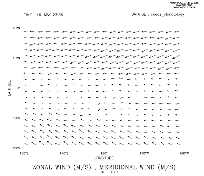
For example (Figure 1_1),
yes? USE coads_climatology !global sea surface data
yes? SET REGION/Z=0/L=5/X=160E:160W/Y=20S:20N
yes? VECTOR uwnd,vwnd !wind velocity vector plot
1.2.1.1 Thinking like a Ferret:
(A discussion on the Ferret outlook on the concepts of data, variables, grids and other basics of Ferret.)
Plottable variables
For this discussion we will coin the term "plottable variables." There are no non-plottable variables that will come up in this discussion but "variables" is a bit too generic. Plottable variables are of 3 types:
- file variables‚ read from disk files
- user-defined variables‚ defined by the LET command
- pseudo-variables‚ regions (I,J,K,L,X,Y,...) used as variables
As much as possible Ferret tries to make all types of variables indistinguishable. All plottable variables are defined on grids. No plottable variables exists in a vacuum for Ferret. The grid on which a plottable variable exists tells how to locate the variable in space and time. In cases where the variables are abstract in nature‚ disconnected from space and time‚ erret will associate those variables with grids that are abstract, too. Where a geographical grid will associate the Nth position along an axis with a location (like 20 degrees north latitude) an abstract grid will simply associate the Nth position with the number N. Plottable variables may be regridded to other grids than the one on which they are defined. (Done with "G=".)
All references to plottable variables must have a complete context. A complete context will be described in detail later. Briefly it means a region in space, an interval in time and the data set(s) in which the variables will be found.
Grids
All Ferret grids are 6-dimensional (Prior to Ferret v6.8, grids were 4-dimensional). In most cases the axes have the obvious interpretation of 3 space coordinates and time, plus two more to allow for e.g. an Ensemble dimension and Forecast-time dimension but sometimes the axes are abstract.
A grid is composed of 6 axes, each describing the coordinates along one dimension. 5d, 4d, 3d, 2d, 1d and 0d grids are regarded as special cases of the full 6 dimensions in which 1 or more axes are set to "NORMAL".
Ferret tries to look at all axes equally‚ the same syntax of regions and transformations applies to each. Calendar dates, east-west longitudes and north-south latitudes are merely convenient ways to format positions along axes that have special interpretations to people‚ not to Ferret. (The only exception to this is that if the Y axis has units of Latitude Ferret will insert cosine(Latitude) factors into some calculations.)
Axes and grids may be defined by "grid files" (which normally have .GRD filename extensions). Axes may also be defined by the DEFINE AXIS command; grids by the DEFINE GRID command.
A context is a region or point in space and time and a data set(s). This is the information needed by Ferret to make sense of a reference to a plottable variable. Suppose that "U" is a variable in a data set (file) called U_DATA. A command like "PLOT U" is meaningful only when Ferret knows that it is supposed to be looking for U in data set U_DATA and knows where in 6-dimensional space it is supposed to plot.
The context space-time region may be described by a mix of subscript and world coordinate positions. Subscripts are specified by I=,J=,K=,L=, M=, N= for axes 1 through 6, respectively. World coordinates are specified by X=,Y=,Z=,T=, E=, F=. On the right of the equal sign a single point may be given or a range specified by low:high may be given. Special formats are allowed for X= (longitude, e.g. 160W), Y=(latitude, e.g. 23.5S) and time (calendar dates like "7-NOV-1989:12:35:00" in quotation marks).
The data set may be given by name or number. The commands SET DATA and CANCEL DATA and the D= context descriptor all accept the name of the data set or its number. The data sets are numbered by the order in which they are pointed to with SET DATA. This order may be seen with SHOW DATA.
You can tell Ferret the context in 3 places:
1. The program context: Using the commands SET REGION and SET DATA you can describe a context in which all commands and expressions will be interpreted. You can look at the program context with SHOW REGION and SHOW DATA. (The command SET DATA is used both to initialize new data sets and to make previously initialized sets the current program context. When SET DATA initializes a new data set that set automatically becomes the data set for the program context.) Example: SET REGION/Z=50
2. The command context: Using the command qualifiers I,J,K,L,X,Y,Z,T and D commands like PLOT,CONTOUR,SHADE,LIST and VECTOR can specify additional context information. Command context information on any axis or on the data set will replace any program context information on the same axis or the data set.
3. The variable context: Using the same qualifiers as the command context any plottable variable name can be modified with additional context information in square brackets (e.g. LET U200 = U[Z=200,D=U_DATA], or LIST U[I=1:100:5]). Variable context information on any axis or the data set will replace any program or command context information on the same axis or the data set.
Transformations
Ferret can transform plottable variables along their axes. Transformations may be specified only in the variable context. Ferret understands a number of transformations that may be specified with the space-time region qualifiers. Some examples: PLOT U[Z=0:100@AVE] ‚ the variable U averaged between Z=0 and Z=100 LIST/L=1:200 U[L=@SBX:5]‚ U with a boxcar smoother of width 5 points along L.
Also,
- @FAV (fill data holes with averages)
- @DIN (definite integral) @IIN (indefinite integral)
- @DDC (centered derivative)
- @SHF (shift data a number of points along an axis)
- @MIN (minimum value along an axis)
... and others (see HELP TRANSFORMATIONS inside Ferret)
1.2.2 Unix command line switches
ferret [-batch <file>.ps][-memsize Mwords] [-unmapped] [-help] [-gif] [-server] [-script journalfile.jnl [arg1] [arg2]...]

or

pyferret [-memsize Mwords] [-nodisplay] [-server] [-quiet] [-script journalfile.jnl [arg1] [arg2]...]
PyFerret has a few options that are different from Ferret switches, see below.
-memsize Mwords
specify the memory (data cache) size in Megawords (default is 25.6)
If memory is severely limited on a system Ferret's default memory cache size may be too large to permit execution. In this case use the "-memsize" qualifier on the command line to specify a smaller cache.
-unmapped
use invisible output windows (useful for creating metafiles when window resizing is needed. You can create metafiles, using any SET WINDOW/SIZE or /ASPECT commands required. Then use gksm2ps to convert to postscript, using gksm2ps options to control orientation and sizing.)
-unmapped is recognized by PyFerret; it has become an alias for the -nodisplay switch, described below.
-help
obtain help on the Unix command line options
-nojnl
start Ferret without a journal file. Within the Ferret session, you can use SET MODE JOURNAL:<filename> to turn on journaling and set the journal file name if desired.
-gif
Ferret can run in batch mode for gif output‚ without an X server (see also -server below). Graphical output is buffered, and is stored in a GIF file by executing the FRAME command. For example:
> ferret -gif
yes? (commands that generate a plot...)
yes? FRAME/FILE=picture.gif
sends the stored graphical output from Ferret to the GIF file picture.gif. Note that the -gif startup mode does NOT take an argument. You can however start Ferret in -batch mode (see below) and specify a gif file name for the output.
Please note the following when using gif mode:
-gif is recognized by PyFerret; it has become an alias for the -nodisplay switch, described below.
- Window resizing only works if the window is cleared before resizing the window. For instance:
yes? set window/clear/size=0.25
will resize the window while if it is issued without /clear,
yes? set window/size=0.8
will result in a blank plot.
- Avoid metafile commands when running in gif mode. In particular,
yes? set mode meta
will result in a warning (NOTE) message and will be ignored.
- Don't create new Ferret windows when running without an X server. The following command:
yes? set window/new
will result in a warning (NOTE) message and will be ignored.
-batch
Ferret can generate PostScript files, gif images, or metafiles without an X server. In a given Ferret session, it will not write more than one type of plot file. (But PyFerret -nodisplay can! See below.) See discussion below for making more than one plot file in the session. If you wish to use this mode, start Ferret with the -batch option:
ferret -batch <file>.ps
ferret -batch <file>.plt
ferret -batch <file>.gif
ferret -batch
where <file> is the name of the output file. Specifying <file>.ps will write postscript files, <file>.gif will write a gif image, and <file>.plt will write metafiles. If "ferret -batch" is given with no file specified, Ferret will write metafiles named metafile.plt.
When the file type is .gif, only the last image that is drawn in the Ferret session is saved as filename.gif. You do not need to issue a FRAME command to save the image.
Please note the following when using PostScript mode:
- The PostScript output will not be fully written to the output file until you exit from Ferret.
- Window sizing commands do not have any effect on PostScript output. (If window sizing is needed, can start Ferret with the -unmapped option, and create metafiles, using any SET WINDOW/SIZE or /ASPECT commands required. Then use gksm2ps to convert to postscript, using gksm2ps options to control orientation and sizing if desired.)
- Any metafile commands when running in PostScript or gif mode will result in a warning (NOTE) message and will be ignored.
- Don't create new Ferret windows when running without an X server. The following command:
yes? set window/new
will result in a warning (NOTE) and will be ignored.
When in batch metafile mode:
A new myfile.plt.~*~ file is started with each new plot "page" that we'd see when running interactively.
SET MODE METAFILE newname.plt will change the name of the metafile to the new name.
The following commands are ignored in metafile batch mode:
- SET MODE METAFILE, except for "SET MODE METAFILE newname.plt". Subsequent metafiles will have the new name.
- CANCEL MODE METAFILE
- SET WINDOW ! except for
- SET WINDOW/ASPECT applies the new aspect ratio
- SET WINDOW/CLEAR starts a new metafile
New plots may be started with these commands when making metafiles:
- New plot command (if we are not in a viewport and not overlaying) PLOT, CONTOUR, SHADE, FILL, VECTOR, CONTOUR, POLYGON, WIRE
- CANCEL VIEWPORT
- SET WINDOW/CLEAR
- PPLUS/RESET
-secure
Run in secure mode -- don't allow SPAWN commands.
-server
Run in server mode -- don't stop on message commands. This mode uses primitive (but faster) command line reading, so it is generally preferred when setting up Ferret from a pipe or batch process. See the notes above under -gif regarding window sizing commands.
-script journalfile.jnl
Run a script, with optional arguments, and exit. Ferret starts, the script runs, and Ferret exits. If Ferret encounters an error, it will issue any error messages and exit to the Unix command line. The switch also sets the -server, -nojnl, and -noverify switches (MODE VERIFY and MODE JOURNAL may be turned back on within the script). It suppresses the banner lines. So that the command line reader can read and process any arguments to the script, -script must be specified last, after any other command-line switches (e.g. -gif or -memsize). Everything listed after the -script journalfile.jnl is taken to be arguments to the script.
> ferret -script file.jnl [arg1] [arg2] [arg3] ...

or

> ferret -gif -memsize 500 -script file.jnl [arg1] [arg2] [arg3]
If a script argument contains spaces, either enclose the argument in double-quotes surrounded by single-quotes; or escape spaces with a backslash.
> pyferret -script file.jnl 7 '"The Title"' '"(my units)"'

or
> pyferret -script file.jnl 7 "The\ Title" "(my\ units)"
PyFerret only
When starting PyFerret, the command switches -memsize, -nojnl, -noverify, -secure, -server, -version, -script, and -help are identical to their behavior in classic Ferret. The -batch switch remains an option but is not recommended. If you use -batch, new windows should not be created and the FRAME command should not be used. In addition the -transparent command line option is not recommended. Instead use the -nodisplay option and the FRAME/FILE=<filename> [ /TRANSPARENT ] command.
-gif and -unmapped are recognized by PyFerret; they are aliases for the -nodisplay switch, listed below. The switch used does not determine the type of plot files that may be saved as is the case for Ferret. We can write any type of plot file when running in -nodisplay mode, or multiple plot types in the same script.
-nodisplay
Do not display to the console; a drawing can be saved using the FRAME command in any of the supported file formats. The /QUALITY option of SET WINDOW will be ignored when this is specified. The deprecated command-line options -unmapped and -gif are aliases of this option.
-quiet
Do not display the startup header.
-python
Start at the Python prompt instead of the Ferret prompt. The ferret prompt can be obtained using 'pyferret.run()'
1.2.3 Sample sessions
This section presents a number of short Ferret sessions that demonstrate common uses. Data sets used in these sessions and throughout this manual are included with the distribution. If Ferret is installed on your system, you can duplicate the examples shown.
1.2.3.1 Accessing a netCDFdata set
In this sample session, the data set "monthly_navy_winds" is specified and certain aspects of it are examined. The command SHOW DATA/VARIABLES displays the variables in "monthly_navy_winds" and where on each axis they are defined. SET REGION specifies where in the grid the user wishes to examine the data. VECTOR produces a vector plot of the indicated variables over the specified region.
yes? USE monthly_navy_winds ! specify the data set
yes? SHOW DATA/VARIABLES ! what's in it?
 currently SET data sets:
 1> /home/porter/tmap/ferret/linux/fer_dsets/data/monthly_navy_winds.cdf (default)

 name title I J K L
 UWND ZONAL WIND 1:144 1:73 ... 1:132
 M/S on grid GDN1 with -99.9 for missing data
 X=18.8E:18.8E(378.8) Y=91.2S:91.2N
 VWND MERIDIONAL WIND 1:144 1:73 ... 1:132
 M/S on grid GDN1 with -99.9 for missing data
 X=18.8E:18.8E(378.8) Y=91.2S:91.2N

 time range: 16-JAN-1982 20:00 to 17-DEC-1992 03:30
1.2.3.2 Reading an ASCII data file
Many examples of accessing ASCII data are available later in this manual. See the chapter, "Data Sets" The simplest access, one variable with one value per record, looks like this:
% ferret
yes? FILE/VARIABLE=v1 snoopy.dat
yes? PLOT v1
yes? QUIT
1.2.3.3 Using viewports
The command SET VIEWPORT allows the user to divide the output graphics "page" into smaller display viewports.
In this sample session, we create two plots in two halves of a window (Figure 1_2):
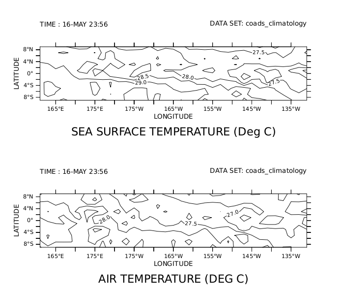
% ferret
yes? USE coads_climatology
yes? SET REGION/X=160E:130W
yes? SET REGION/Y=-10:10/L=5
yes? SET VIEWPORT upper
yes? CONTOUR sst
yes? SET VIEWPORT lower
yes? CONTOUR airt
yes? QUIT
1.2.3.4 Using abstract variables
Abstract variables (expressions that contain no dependencies on disk-resident data) can be easily displayed with Ferret. See the chapter "Variables and Expressions", section Abstract variables, for several examples and detailed information.
For example, a user wishing to examine the function SIN(X) on the interval [0,3.14] might use (Figure 1_3):
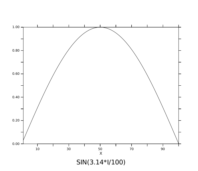
% pyferret
yes? PLOT/I=1:100 sin(3.14*I/100)
yes? QUIT
A transformation is an operation performed on a variable along a particular axis and is specified with the syntax "@trn" where "trn" is the name of a transformation. See the chapter "Variables and Expressions", section Transformations, for detailed information.
A user may wish to look at ocean temperatures averaged over a range of depths. In this sample session, we look at temperatures averaged from 0 to 100 meters of depth using a data set which has detailed resolution in depth (Figure 1_4). We plot the data along longitude 160 west from latitude 30 south to 30 north.

% ferret
yes? USE levitus_climatology
yes? SET REGION/Y=30s:30n/X=160W
yes? PLOT temp[Z=0:100@AVE]
yes? QUIT
1.2.3.6 Using algebraic expressions
See the chapter "Variables and Expressions", section Expressions for a description of valid expressions.
In this example, the data set contains raw sea surface temperatures, air temperatures, and wind speed measurements. We wish to look at a shaded plot of sensible heat at its first timestep (L=1) (Figure 1_5). We specify a latitude range and contour levels.
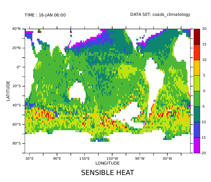
% ferret
yes? USE coads_climatology !monthly COADS climatology
yes? LET kappa = 1 !arbitrary
yes? LET/TITLE="SENSIBLE HEAT" sens_heat = kappa * (airt-sst) * wspd
yes? SHADE/L=1/LEV=(-20,20,5)/Y=-90:40 sens_heat
yes? QUIT
1.2.3.7 Finding the 20-degree isotherm
Isotherms can be located with the "@LOC" transform, which returns the axis location where the value of the argument of @LOC first occurs. Thus, "TEMP[Z=0:200@LOC:20]" locates the first occurrence of the temperature value 20 along the Z axis, scanning all the data between 0 and 200 meters.
A session examining the 20-degree isotherm in mid-Pacific ocean data (Figure 1_6):
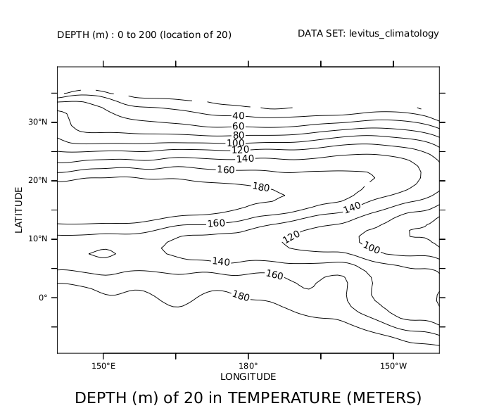
% ferret
yes? USE levitus_climatology
yes? SET REG/Y=10s:40n/X=140E:140W
yes? CONTOUR/SIZE=0.12 temp[Z=0:200@LOC:20]
yes? QUIT
Note that the transformation @WEQ could have been used to display ANY variable on the surface defined by the 20 degree isotherm.