PyFerret/Ferret v7.6 implement automated handling of the Discrete Sampling Geometries standard in netCDF-CF. See Chapter 9 of the CF standard for the details.
Attributes in the file informs Ferret that this is a Feature Collection organized as a Discrete Sampling Geometries dataset. The data is often the output of an ERDDAP tabledap datset, using "save as .ncCF". A "Feature" is a single Timeseries, Profile, Trajectory or Point. A Feature Collection contains one or more Features in the file. The files are organized as Discrete Sampling Geometry Contiguous ragged-array files, following the CF Standard for Discrete Sampling Geometries.
The datasets used in this demo are included for the current FerretDatasets Distribution
Here's how it looks: Run the script dsg_tutorial.jnl
> pyferret
yes? go dsg_tutorial
********************************************************************
Timeseries Feature Type
********************************************************************
yes? use dsg_timeseries_example.nc
yes? show data
     currently SET data sets:
    1> /home/users/tmap/ferret/linux/fer_dsets/data/dsg_timeseries_example.nc  (default)
       DSG Feature type Timeseries
 name     title                             I         J         K         L         M         N
 STATION  Station                          ...       ...       ...       ...       1:70      ...
 ROWSIZE  Number of Observations for this  ...       ...       ...       ...       1:70      ...
 LONGITUDE
          Nominal Longitude                ...       ...       ...       ...       1:70      ...
 LATITUDE Nominal Latitude                 ...       ...       ...       ...       1:70      ...
 ARRAY    Array                            ...       ...       ...       ...       1:70      ...
 WMO_PLATFORM_CODE
          WMO Platform Code                ...       ...       ...       ...       1:70      ...
 DEPTH    Depth                            ...       ...       ...     tot 2376    1:70      ...
 TIME     Centered Time                    ...       ...       ...     tot 2376    1:70      ...
 T_25     Sea Surface Temperature          ...       ...       ...     tot 2376    1:70      ...
 QT_5025  Sea Surface Temperature Quality  ...       ...       ...     tot 2376    1:70      ...
Internally Ferret creates a “translation” grid based upon the units and coordinate range for the coordinates for each relevant direction in the dataset, which allows the gridded coordinate formatting routines to be used for DSG variables. The output of SHOW DATA/FULL command includes extreme coordinate limits of the coordinates in the data set, as does SHOW GRID.
yes? show grid t_25
    GRID (G004)
 DSG Feature type Timeseries
 name       axis              # pts   start                end                 subset
 normal    X
 normal    Y
 normal    Z
 FEATURE_T TIME              2376 r   15-JAN-2017 12:00    21-APR-2017 12:00   Variable lengths
 FEATURES  E (instance)        70 r   1                    70                  full
 normal    F

Dataset coordinates:
  longitude range: 0E to 10W
  latitude range: 19S to 21N
  depth range: 1 to 1.5
  time range: 15-JAN-2017 12:00 to 21-APR-2017 12:00
********************************************************************
Graphics
********************************************************************
Each feature type has a native plot type “PLOT VAR” will plot the variable in the currently selected set of features.
First lets make a map showing the locations of the stations. This is nothing new, we draw a map and overlay the locations with PLOT/VS
yes? go basemap x=140:360 y=-40:40 20
yes? plot/vs/over/nolabel/color=blue/symbol=19/siz=0.2/thick longitude, latitude

Now plot the temperature variable for all of the time series in the collection at once. They are all plotted together, with a line key limited automatically to 40 of the lines (as is also done for many lines in any other plot). Ferret understands DSG coordinates internally, much as it would understand gridded coordinates. So the plot is properly formatted and self-describing.
yes? plot t_25
           *** NOTE: Too many lines to label. Labeling initial 40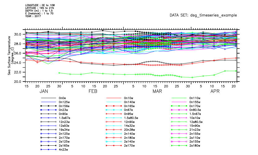
********************************************************************
Constraints
********************************************************************
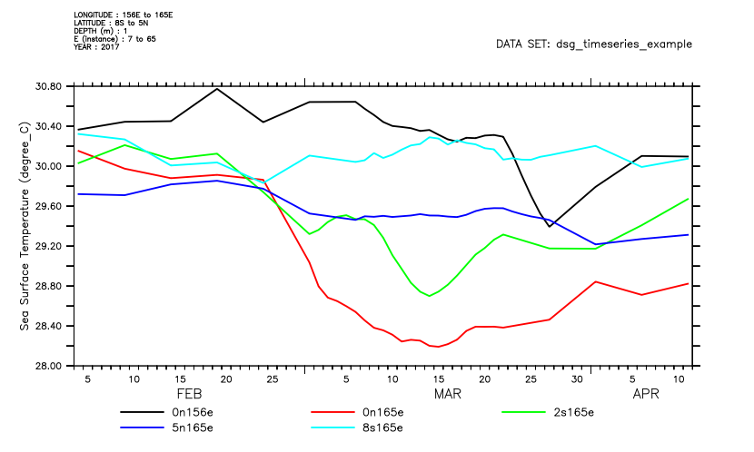
Ordinary PyFerret qualifiers for coordinate limits, /X=, /Y=, /Z=, /T=, /E= operate as they do with a gridded dataset -- i.e. they control the region displayed by the graphics and the data that gets plotted or listed.
yes? plot/thick/x=130e:170e/y=8s:5n/T=1-FEB-2017:15-APR-2017 T_25
********************************************************************
Masking
********************************************************************
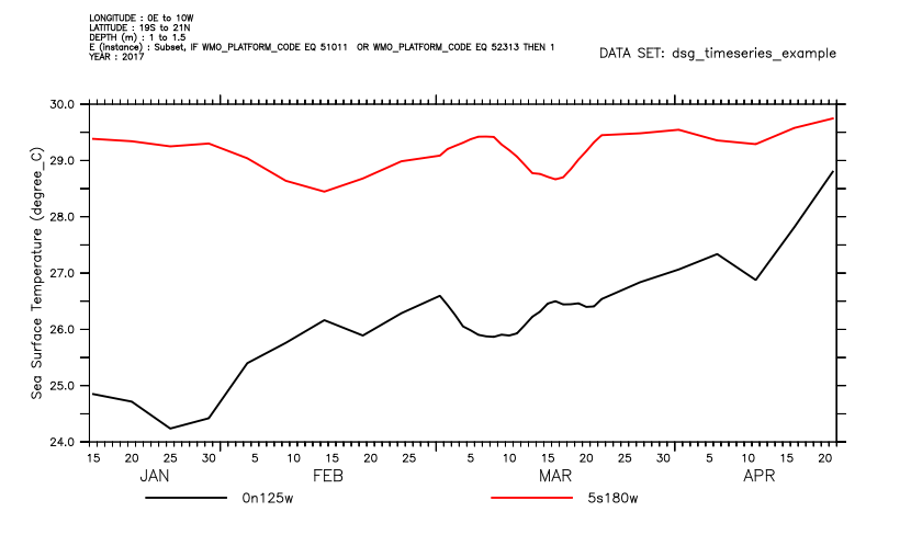
To select features (individual time series, profiles or trajectories) define a feature-mask. SET DATA/FMASK= (or USE/FMASK=) applies the mask to the dataset until it is canceled. A listing shows what mask is in place, and lists the data selected.
yes? let wmo_mask = IF wmo_platform_code EQ 51011 \
yes?  OR wmo_platform_code EQ 52313 then 1

yes? use/fmask=wmo_mask dsg_timeseries_example.nc

yes? list/t=1-jan-2017:25-feb-2017 t_25
   DATA SET: /home/users/tmap/ferret/linux/fer_dsets/data/dsg_timeseries_example.nc
Mask on features has been set: IF WMO_PLATFORM_CODE EQ 51011  OR WMO_PLATFORM_CODE EQ 52313 THEN 1
   SUBSET   : TIME: 15-JAN-2017 12:00 to 24-FEB-2017 12:00
 STATION    is Timeseries-id
 T_25       is Sea Surface Temperature (degree_C)
    FEATURE  STATION     LONGITUDE  LATITUDE   DEPTH            TIME        T_25

     4           0n125w       125W         0       1   15-JAN-2017 12:00   24.85
     4           0n125w       125W         0       1   20-JAN-2017 12:00   24.72
     4           0n125w       125W         0       1   25-JAN-2017 12:00   24.24
     4           0n125w       125W         0       1   30-JAN-2017 12:00   24.42
     4           0n125w       125W         0       1   04-FEB-2017 12:00   25.40
     4           0n125w       125W         0       1   09-FEB-2017 12:00   25.76
     4           0n125w       125W         0       1   14-FEB-2017 12:00   26.16
     4           0n125w       125W         0       1   19-FEB-2017 12:00   25.89
     4           0n125w       125W         0       1   24-FEB-2017 12:00   26.29

    54           5s180w       180E        5S       1   15-JAN-2017 12:00   29.38
    54           5s180w       180E        5S       1   20-JAN-2017 12:00   29.34
    54           5s180w       180E        5S       1   25-JAN-2017 12:00   29.25
    54           5s180w       180E        5S       1   30-JAN-2017 12:00   29.30
    54           5s180w       180E        5S       1   04-FEB-2017 12:00   29.04
    54           5s180w       180E        5S       1   09-FEB-2017 12:00   28.64
    54           5s180w       180E        5S       1   14-FEB-2017 12:00   28.45
    54           5s180w       180E        5S       1   19-FEB-2017 12:00   28.68
    54           5s180w       180E        5S       1   24-FEB-2017 12:00   28.99

yes? plot/thick t_25
********************************************************************
Other Feature-types:
Timeseries, Profile, Trajectory and Point types
are currently implemented.
********************************************************************
********************************************************************
Profiles
********************************************************************
Profile datasets, like timeseries, are drawn as lines of data at a collection of stations. The legend labels are the profile station ID’s from the file. Subsetting and masking is done in the same way as for timeseries data.
yes? use dsg_profile_example
yes? show data
     currently SET data sets:
    1> /home/users/tmap/ferret/linux/fer_dsets/data/dsg_profile_example.nc  (default)
       DSG Feature type Profile
name     title                             I         J         K         L         M         N
ID       profile id                       ...       ...       ...       ...       1:30      ...
ROWSIZE  Number of Observations for this  ...       ...       ...       ...       1:30      ...
LONGITUDE
          station longitude                ...       ...       ...       ...       1:30      ...
LATITUDE station latitude                 ...       ...       ...       ...       1:30      ...
DEPTH    Depth                            ...       ...     tot 1268    ...       1:30      ...
TIME     Time                             ...       ...       ...       ...       1:30      ...
TEMP     Temperature                      ...       ...     tot 1268    ...       1:30      ...
SAL      Salinity                         ...       ...     tot 1268    ...       1:30      ...
SIGMA_T  Sigma-T                          ...       ...     tot 1268    ...       1:30      ...

yes? plot/thick sigma_t
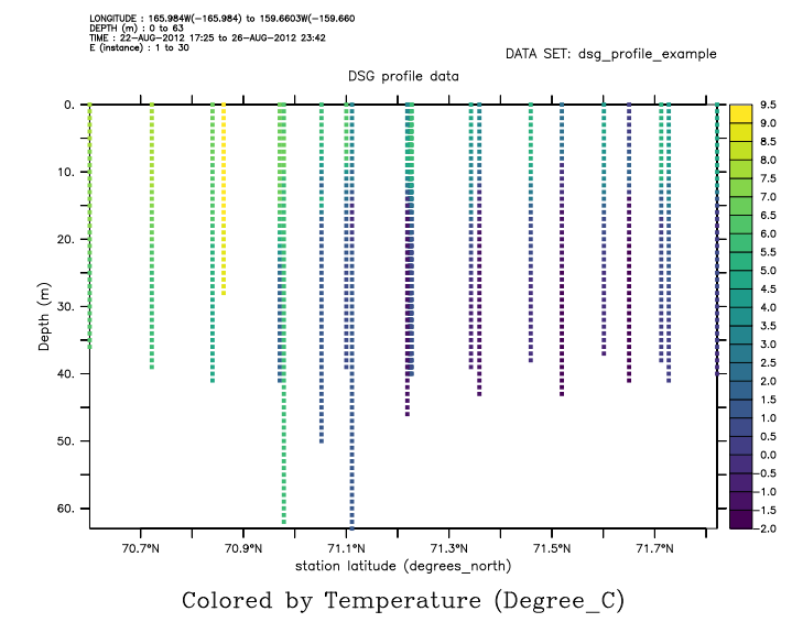
Another plot style uses the RIBBON/VS plot command, with 3 arguments: the locations in two directions, and the variable to use for color. Time on the horizontal axis will result in a formatted time axis. Or specify longitude or latitude on the horizontal axis.
yes? ribbon/thick/vs latitude, depth, temp
********************************************************************
Trajectories
********************************************************************
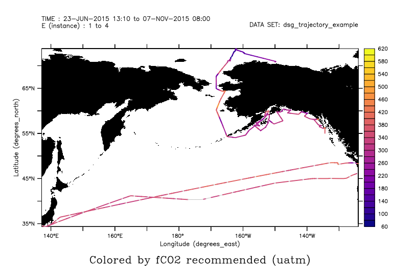
Trajectory data has longitude, latitude, time, depth, and measurements along the trajectory paths. The native plot type is a ribbon plot, location colored by measurement. The PLOT command automatically draws a ribbon plot. The usual plot qualifiers apply, setting color levels, palette, and so on. Utility scripts such as "GO LAND" or GO FLAND" work as always.
yes? use dsg_trajectory_example.nc
yes? plot/thick/palette=plasma fco2_recommended
yes? go fland 5 black
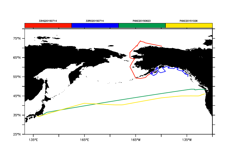
Or, color by the trajectory ID, so that each one has a color. If there are few enough trajectories, the ID's become the labels along the colorbar.
yes? go basemap x=130:240 y=25:80 5 black
yes? plot/over/nolabel/thick/palette=ten_by_levels/key=horiz expocode
********************************************************************
Working with trajectory data as time series
********************************************************************
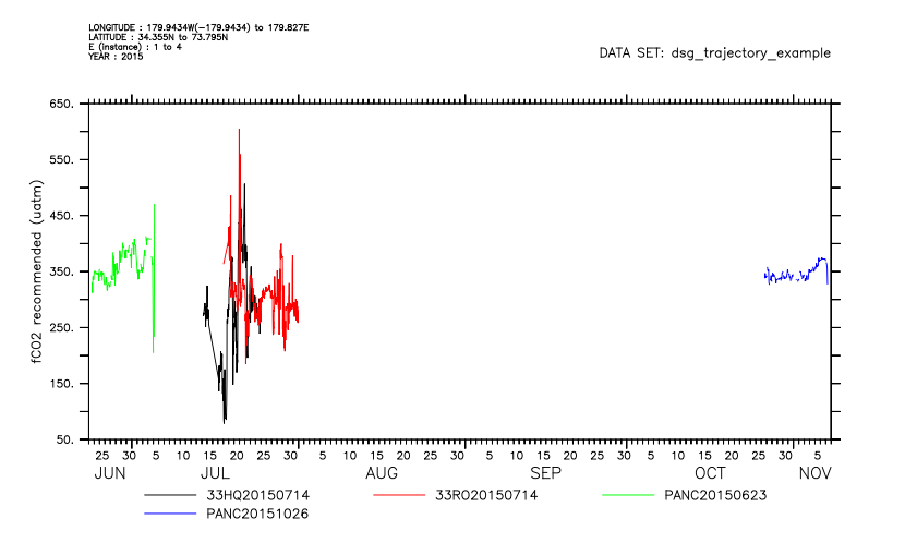
For each observation along a trajectory we have a time coordinate as well as longitude and latitude. This means the data can be interpreted as a set of time series. Change to a timeseries interpretation with USE/FEATURETYPE. This can be applied when first opening the data or on an open dataset.
yes? use/featuretype=timeseries dsg_trajectory_example.nc
yes? plot fco2_recommended
And for any DSG dataset, we can ignore the DSG-specific elements of the file and handle it as we would have prior to PyFerret v7.6. Note how the grid is now just count-of-observations, and the plot has no information about the coordinates. We no longer have automatic masking-by-feature and constraints-by-world coordinate
yes? use/feature=none dsg_trajectory_example.nc
yes? show data
     currently SET data sets:
    1> /home/users/tmap/ferret/linux/fer_dsets/data/dsg_trajectory_example.nc  (default)
 name     title                             I         J         K         L         M         N
 EXPOCODE expocode                         ...       ...       ...       ...       1:4       ...
 ROWSIZE  Number of Observations for this  ...       ...       ...       ...       1:4       ...
 LONGITUDE
          Longitude                        1:1326    ...       ...       ...       ...       ...
 LATITUDE Latitude                         1:1326    ...       ...       ...       ...       ...
 TIME     Time                             1:1326    ...       ...       ...       ...       ...
 FCO2_RECOMMENDED
          fCO2 recommended                 1:1326    ...       ...       ...       ...       ...
 TEMPERATURE_EQUI
          equilibrator chamber temperatur  1:1326    ...       ...       ...       ...       ...


yes? plot temperature_equi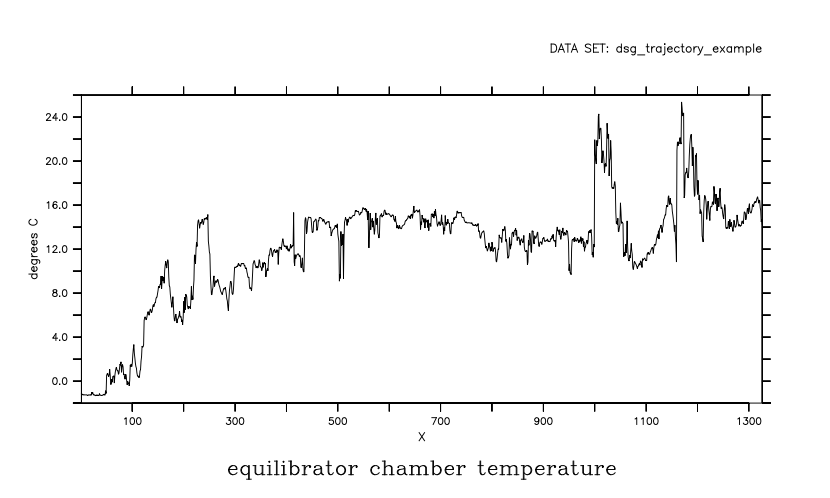
To turn off automated DSG-handling for the rest of the session, issue a "CANCEL MODE DSG" command.
********************************************************************
Points
********************************************************************
Let's take a quick look at Point data. The plot type is a "ribbon" plot, locating the data in X-Y.
yes? use dsg_point_example
yes? show data
     currently SET data sets:
    1> /home/users/tmap/ferret/linux/fer_dsets/data/dsg_point_example.nc  (default)
       DSG Feature type Point
 name     title                             I         J         K         L         M         N
 LATITUDE Latitude                         ...       ...       ...       ...     tot 1158    ...
 LONGITUDE
          Longitude                        ...       ...       ...       ...     tot 1158    ...
 TIME     Start Time                       ...       ...       ...       ...     tot 1158    ...
 STATION  Station                          ...       ...       ...       ...     tot 1158    ...
 COMMON_NAME
          Common Name                      ...       ...       ...       ...     tot 1158    ...
 LARVAE_SIZE
          Total length of the larvae       ...       ...       ...       ...     tot 1158    ...
 LARVAE_COUNT
          Raw count of larvae              ...       ...       ...       ...     tot 1158    ...


yes? plot/thick/lev=v larvae_size
yes? go land_detail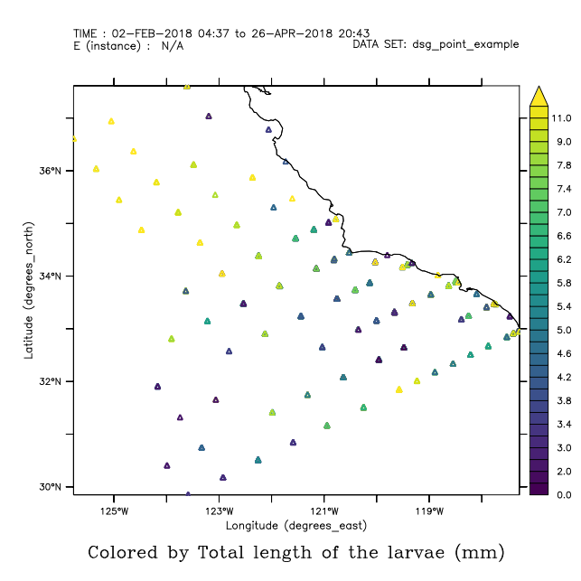
********************************************************************
Changing gears now, from graphics to some of the analysis operations we might do with any dataset.
The syntax for constraints and masking is used here as well.
********************************************************************
********************************************************************
Writing subsets
********************************************************************
The SAVE command writes new DSG files containing subsets of DSG datasets. The elements of the DSG file including the ID and coordinate data are automatically written when an observed data variable is written, so the result is a valid DSG file. Use qualifiers or a mask to subset data.
yes? use dsg_timeseries_example
yes? save/clobber/file=my_southern_stations.nc/x=0:180/y=-20:0 t_25

yes? use my_southern_stations.nc
yes? show data
     currently SET data sets:
    1> /home/users/tmap/ferret/linux/fer_dsets/data/dsg_timeseries_example.nc
       DSG Feature type Timeseries
 name     title                             I         J         K         L         M         N
 STATION  Station                          ...       ...       ...       ...       1:70      ...
 ROWSIZE  Number of Observations for this  ...       ...       ...       ...       1:70      ...
 LONGITUDE
          Nominal Longitude                ...       ...       ...       ...       1:70      ...
 LATITUDE Nominal Latitude                 ...       ...       ...       ...       1:70      ...
 ARRAY    Array                            ...       ...       ...       ...       1:70      ...
 WMO_PLATFORM_CODE
          WMO Platform Code                ...       ...       ...       ...       1:70      ...
 DEPTH    Depth                            ...       ...       ...     tot 2376    1:70      ...
 TIME     Centered Time                    ...       ...       ...     tot 2376    1:70      ...
 T_25     Sea Surface Temperature          ...       ...       ...     tot 2376    1:70      ...
 QT_5025  Sea Surface Temperature Quality  ...       ...       ...     tot 2376    1:70      ...

    2> ./my_southern_stations.nc  (default)
       DSG Feature type Timeseries
 name     title                             I         J         K         L         M         N
 STATION  Station                          ...       ...       ...       ...       1:21      ...
 ROWSIZE  Number of Observations for this  ...       ...       ...       ...       1:21      ...
 LONGITUDE
          Nominal Longitude                ...       ...       ...       ...       1:21      ...
 LATITUDE Nominal Latitude                 ...       ...       ...       ...       1:21      ...
 DEPTH    Depth                            ...       ...       ...     tot 757     1:21      ...
 TIME     Centered Time                    ...       ...       ...     tot 757     1:21      ...
 T_25     Sea Surface Temperature          ...       ...       ...     tot 757     1:21      ...
Currently we can APPEND new variables of the same size to a dataset, but appending further features or extending the dataset, for instance in time, is not now implemented.
********************************************************************
User-defined variables
********************************************************************
Standard LET syntax defines new variables based on DSG data.
yes? use/feature=timeseries dsg_trajectory_example.nc
yes? let/like=temperature_equi/units="K" temp_k = temperature_equi + 273.13
yes? plot/t=15-jun-2015:10-aug-2015 temp_k
********************************************************************
Transformations
********************************************************************
Transformations apply within each feature, not over the whole file or region.
Returning to our timeseries dataset, compute the maximum temperature reached and the number of valid data in each time series during Jan-March of 2017
yes? use dsg_timeseries_example

yes? LET t_max = t_25[T=1-JAN-2017:31-Mar-2017@MAX]
yes? LET t_ngood = t_25[T=1-JAN-2017:31-MAR-2017@NGD]

yes? list/M=1:15 t_max, t_ngood
   DATA SET: /home/users/tmap/ferret/linux/fer_dsets/data/dsg_timeseries_example.nc
   SUBSET   : E (instance): 1 to 15
 STATION    is Timeseries-id
 T_25       is Sea Surface Temperature (degree_C) (maximum, each Timeseries)
 T_25       is Sea Surface Temperature (number of valid, each Timeseries)
    FEATURE  STATION     LONGITUDE  LATITUDE    T_25    T_25
     1             0n0e         0E         0   29.83   32.00
     2            0n10w        10W         0   29.64   32.00
     3           0n110w       110W         0   27.63   23.00
     4           0n125w       125W         0   26.84   32.00
     5           0n140w       140W         0   26.89   32.00
     6           0n155w       155W         0   27.39   32.00
     7           0n156e       156E         0   30.77   32.00
     8           0n165e       165E         0   30.40   32.00
     9           0n170w       170W         0   27.20   32.00
    10            0n23w        23W         0   28.87   28.00
    11            0n67e        67E         0   30.26   32.00
    12          0n80.5e      80.5E         0   30.14   32.00
    13            0n90e        90E         0   29.64   22.00
    14            0n95w        95W         0   28.60   32.00
    15          1.5n67e        67E      1.5N   30.19   32.00
Now list a subset of the running-sum transformation for our profile data. Note that the sums start over with each new profile.
yes? use dsg_profile_example
yes? list/m=3:5/z=1:6/prec=6 sal, sal[z=@rsum]
   DATA SET: /home/users/tmap/ferret/linux/fer_dsets/data/dsg_profile_example.nc
   DSG profile data
   SUBSET   : DEPTH (m): 1 to 6 (running sum)
              E (instance): 3 to 5
 ID         is Profile-id-id
 SAL        is Salinity (PSU)
 SAL        is Salinity (PSU) (running sum, each Profile-id)
    FEATURE  ID          LONGITUDE  LATITUDE   DEPTH            TIME          SAL      SAL

     3       aq1201c033  164.2148W   71.223N       1   23-AUG-2012 04:01  29.9012    59.80
     3       aq1201c033  164.2148W   71.223N       2   23-AUG-2012 04:01  29.9012    89.70
     3       aq1201c033  164.2148W   71.223N       3   23-AUG-2012 04:01  29.9018   119.61
     3       aq1201c033  164.2148W   71.223N       4   23-AUG-2012 04:01  29.9020   149.51
     3       aq1201c033  164.2148W   71.223N       5   23-AUG-2012 04:01  29.9021   179.41
     3       aq1201c033  164.2148W   71.223N       6   23-AUG-2012 04:01  29.9261   209.34

     4       aq1201c034  164.2087W   71.226N       1   23-AUG-2012 08:08  29.8438    59.69
     4       aq1201c034  164.2087W   71.226N       2   23-AUG-2012 08:08  29.8438    89.53
     4       aq1201c034  164.2087W   71.226N       3   23-AUG-2012 08:08  29.8438   119.38
     4       aq1201c034  164.2087W   71.226N       4   23-AUG-2012 08:08  29.8532   149.23
     4       aq1201c034  164.2087W   71.226N       5   23-AUG-2012 08:08  29.8997   179.13
     4       aq1201c034  164.2087W   71.226N       6   23-AUG-2012 08:08  29.8747   209.00

     5       aq1201c035  164.2018W   71.224N       1   23-AUG-2012 12:26  29.6829    59.37
     5       aq1201c035  164.2018W   71.224N       2   23-AUG-2012 12:26  29.6829    89.05
     5       aq1201c035  164.2018W   71.224N       3   23-AUG-2012 12:26  29.6732   118.72
     5       aq1201c035  164.2018W   71.224N       4   23-AUG-2012 12:26  29.6771   148.40
     5       aq1201c035  164.2018W   71.224N       5   23-AUG-2012 12:26  29.6801   178.08
     5       aq1201c035  164.2018W   71.224N       6   23-AUG-2012 12:26  29.7267   207.81
********************************************************************
Regridding to a common time or vertical axis
********************************************************************
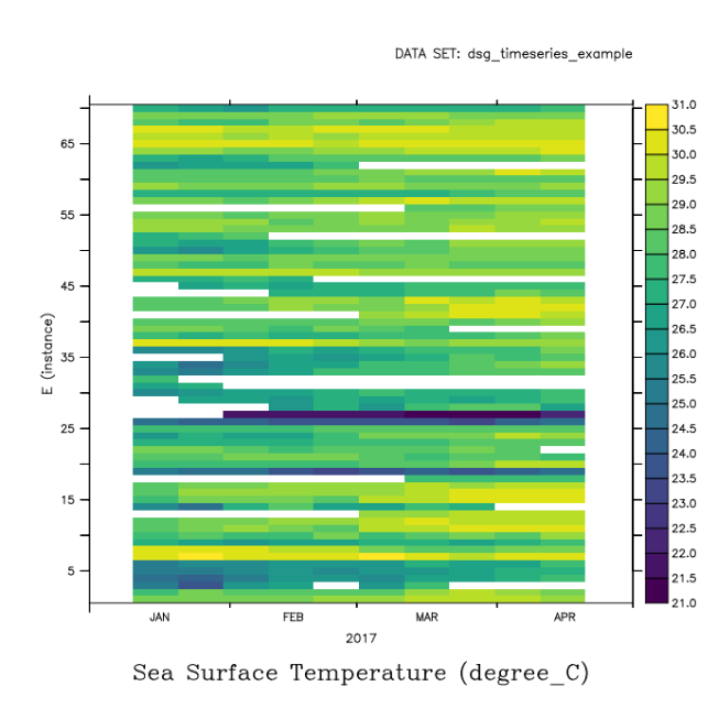
A set of timeseries or profiles in a DSG dataset may not have a common set of time coordinates or Z levels, respectively. The set of timeseries or set of profiles can be regridded to a common time or z axis using an ordinary regridding operation. The result is a 2-D grid of data in T and E for a timeseries, or Z and E for Profile data, Feature-number vs common axis.
SHOW GRID output has shown us that the dataset has a time range of January to April 2017. We can use any time interval.
yes? use dsg_timeseries_example
yes? define axis/t="15-jan-2017:12:00":"21-apr-2017:12:00":10/unit=days tuniform
yes? let/like=t_25 t_25_station_vs_time = t_25[gt=tuniform]
yes? shade t_25_station_vs_time
********************************************************************
Comparisons with gridded data
********************************************************************
DSG data differencing with model or other gridded data: sample data from a grid at the times and locations of the DSG data
To sample data from the model grid, define a regridding operation, G= to "regrid" a variable on a rectangular grid onto the coordinate collection implied by a Discrete Sampling Geometry, the locations and times of the station data.
Open a reference gridded dataset and compare the potential temperature data with the TAO buoy Timeseries data.
yes? use dsg_timeseries_example
yes? use http://www.esrl.noaa.gov/psd/thredds/dodsC/Datasets/ncep.reanalysis/surface/pottmp.sig995.2017.nc

yes? show data 2
     currently SET data sets:
    2> http://www.esrl.noaa.gov/psd/thredds/dodsC/Datasets/ncep.reanalysis/surface/pottmp.sig995.2017.nc  (default)

 name     title                             I         J         K         L
 POTTMP   4xDaily potential temperature a  1:144     1:73      ...       1:1460


show grid t_25[d=1]
    GRID (G004)
 DSG Feature type Timeseries
 name       axis              # pts   start                end                 subset
 normal    X
 normal    Y
 normal    Z
 FEATURE_T TIME              2376 r   15-JAN-2017 12:00    21-APR-2017 12:00   Variable lengths
 FEATURES  E (instance)        70 r   1                    70                  full
 normal    F

Dataset coordinates:
  longitude range: 0E to 10W
  latitude range: 19S to 21N
  depth range: 1 to 1.5
  time range: 15-JAN-2017 12:00 to 21-APR-2017 12:00


yes? show grid pottmp[d=2]
    GRID GOJ1
 name       axis              # pts   start                end                 subset
 LON       LONGITUDE          144mr   0E                   2.5W                full
 LAT       LATITUDE            73 r   90S                  90N                 full
 normal    Z
 TIME      TIME              1460 r   01-JAN-2017 00:00    31-DEC-2017 18:00   full
Plot the gridded data sampled at the DSG space-time coordinates. Note that if the amount of model data that must be accessed
is large, Ferret dynamic memory management will read the data and compute the result in pieces.
yes? let/like=pottmp[d=2] pottmp_at_buoys = pottmp[d=2,g=t_25[d=1]]


yes? list/x=140w/y=0/t=15-jan-2017:15-feb-2017 t_25[d=1], pottmp_at_buoys
   DATA SET: /home/users/tmap/ferret/linux/fer_dsets/data/dsg_timeseries_example.nc
   SUBSET   : LONGITUDE: 140W
              LATITUDE: 0
              TIME: 15-JAN-2017 12:00 to 14-FEB-2017 12:00
 STATION         is Timeseries-id
 T_25            is Sea Surface Temperature (degree_C)
 POTTMP_AT_BUOYS is 4xDaily potential temperature at sigma level 995 (degK)
    FEATURE  STATION     LONGITUDE  LATITUDE   DEPTH            TIME        T_25 POTTMP_AT_BUOYS

     5           0n140w       140W         0       1   15-JAN-2017 12:00   25.25   297.1
     5           0n140w       140W         0       1   20-JAN-2017 12:00   25.37   297.8
     5           0n140w       140W         0       1   25-JAN-2017 12:00   25.48   297.7
     5           0n140w       140W         0       1   30-JAN-2017 12:00   25.54   297.6
     5           0n140w       140W         0       1   04-FEB-2017 12:00   25.57   299.1
     5           0n140w       140W         0       1   09-FEB-2017 12:00   25.72   297.8
     5           0n140w       140W         0       1   14-FEB-2017 12:00   26.04   296.9
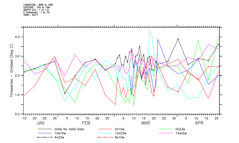
Compute the difference between observed and gridded values.
Define a variable to sample the gridded variable "pottmp" at the station locations and times of the timeseries collection. The NCEP temperature is in Degrees K, so convert to C.
yes? let sampled_t = pottmp[d=2,g=t_25[d=1]] - 273.15

Now define a variable with the difference between the timeseries observations and the sampled grid.
yes? let/title="Timeseries - Gridded"/units="Deg C" diff = t_25[d=1] - sampled_t
And finally plot the difference for the timeseries stations that are located in the Atlantic Ocean.
yes? plot/x=300:360/y=-15:15 diff
dsg_tutorial is now completed.


