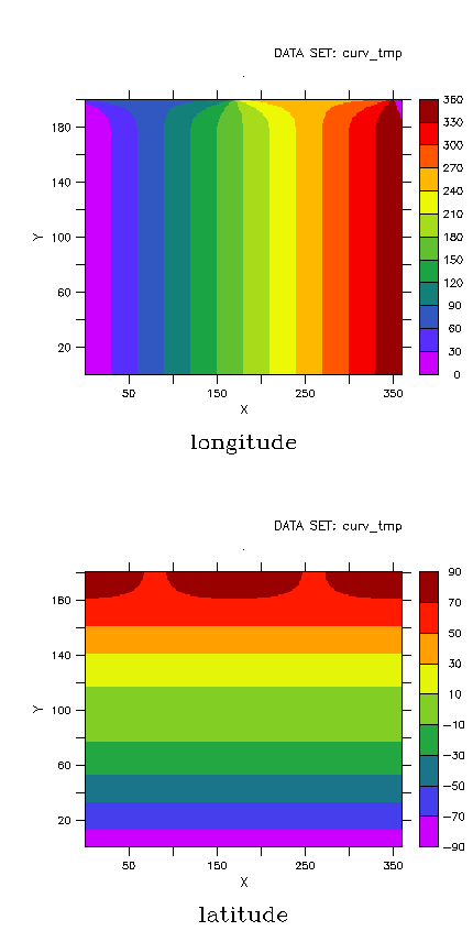
By "curvilinear coordinate data" we refer to data which is curvilinear in the XY plane there. We presume that the X,Y coordinates (typically longitude, latitude) are available through other dependent variables.

Here is an example showing a curvilinear grid, taken from http://www.wldelft.nl/rnd/intro/topic/2003-swe/.

Curvilinear data may be defined by a map projection, or by data in a file that has a curvilinear grid. A curvilinear grid has longitudes and latitudes defined by coordinates (lon[i, j],lat[i, j]) in 2D, and the data fields are also defined on the [i,j] index grid. In the CF standard for netCDF files at  http://cf-pcmdi.llnl.gov, these grids are discussed in the section titled " Two-dimensional latitude, longitude coordinate variables". The netCDF header for a file containing data on a curvilnear grid looks like this (when viewed with the Unix command ncdump -h). Note how the coordinate variables lon and lat are 2-D fields. The coordinate variables and the data field tmp share a grid in index space.

dimensions:
 xc = 180 ;
 yc = 173 ;
variables:
 float xc(xc) ;
   xc:long_name = "x-index in Cartesian system" ;
   xc:units = "m" ;
 float yc(yc) ;
   yc:long_name = "y-index in Cartesian system" ;
   yc:units = "m" ;
 float lon(yc,xc) ;
   lon:long_name = "longitude" ;
   lon:units = "degrees_east" ;
 float lat(yc,xc) ;
   lat:long_name = "latitude" ;
   lat:units = "degrees_north" ;
 tmp:long_name = "temperature" ;
   tmp:units = "K" ;
   tmp:coordinates = "lon lat" ;

When such a dataset is opened in Ferret, the output of a SHOW DATA command will look like:

yes? show data
    currently SET data sets:
   1> ./tmp.nc  (default)
name     title   I         J         K         L
TMP temperature 1:180     1:173     ...       ...
LON longitude   1:180     1:173     ...       ...
LAT longitude   1:180     1:173     ...       ...

This data can be plotted with the 3-argument SHADE, FILL or CONTOUR commands

yes? SHADE tmp, lon, lat

You can see what the grid looks like by doing a shade plot of the coordinate variables:

yes? set view ul; shade lon
yes? set view ll; shade lat

8.8.1 Visualization techniques for curvilinear coordinate data

Visualizations of curvilinear coordinate data in the XY plane section planes are best handled with the 3-argument versions of the SHADE, FILL, and Contour commands. See further information in the chapter "Customizing Plots".

For visualization of curvilinear coordinate data in other planes or orientations use the techniques described under "Analysis techniques for curvilinear coordinate data."

8.2.2 Analysis techniques for curvilinear coordinate data

Analysis of curvilinear coordinate data may be done in the curvilinear coordinate system or in a rectilinear (including lat-long) coordinate system. If the analysis is done in the curvilinear coordinate system, it is the responsibility of the user to ensure that the proper geometric factors are applied when integrals and derivatives are computed. Converting other fields to the curvilinear coordinate system is most easily accomplished with the function RECT_TO_CURV. Curvilnear grids may be converted to rectilinear grids using the functions CURV_TO_RECT_MAP and CURV_TO_RECT.